Concavity and the second derivative test (Calc 1; Lecture 2-8; Fall 26)

Overview

The lecture connects the first derivative to increasing and decreasing behavior, then develops concavity through the second derivative and uses sign charts to locate inflection points. It compares the first and second derivative tests for classifying critical points, working through polynomial and exponential examples including x³ − 3x² − 9x + 15 and 9x e^(−x²/6).

Key takeaways

A positive second derivative means the first derivative is increasing and the curve is concave up; a negative second derivative means the first derivative is decreasing and the curve is concave down.
A zero or undefined second derivative marks only a possible inflection point; verify that the second derivative changes sign across the candidate.
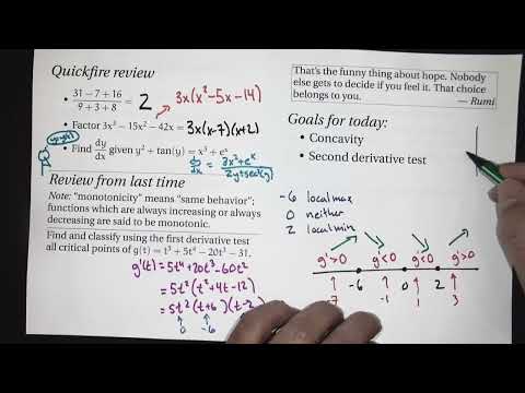
For g(t) = t⁵ + 5t⁴ − 20t³ − 31, the first derivative signs classify −6 as a local maximum, 0 as neither, and 2 as a local minimum.
Even-multiplicity factors such as x² may leave a sign unchanged across a root, as at x = 0 in 60x²(x + 1)(x − 3); that root is not an inflection point without a concavity change.
The exponential e^(−x²/6) is always positive, so in f″(x) = x e^(−x²/6)(x² − 9), the sign chart depends only on x and x² − 9.
The second derivative test classifies a critical point as a local minimum when f″ is positive and a local maximum when f″ is negative; f″ = 0 leaves the classification inconclusive.

Chapters

0:00 Quick Review: Factoring and Implicit Differentiation

The opening arithmetic review evaluates a fraction with numerator 31 − 7 + 16 and denominator 9 + 3 + 8 as 2.
Factor 3x³ − 15x² − 42x by first extracting 3x, then factoring x² − 5x − 14 as (x − 7)(x + 2).
Implicit differentiation applies when an equation mixes x and y without isolating y; treat y as a function of x and use the chain rule.

3:57 Monotonicity and Finding Critical Points

Monotonicity means a function maintains one behavior—consistently increasing or consistently decreasing—over an interval.
The first derivative identifies increasing and decreasing behavior through its sign: positive means increasing, negative means decreasing.
For g(t) = t⁵ + 5t⁴ − 20t³ − 31, the derivative is 5t²(t + 6)(t − 2), giving critical numbers −6, 0, and 2.

8:20 First Derivative Sign Chart: Maxima, Minima, and Neither

Test g′(t) on the intervals separated by −6, 0, and 2, using sample values such as −7, −1, 1, and 3.
The derivative signs are positive, negative, negative, and positive, respectively, so the function rises, falls, falls, then rises.
The first derivative test classifies t = −6 as a local maximum, t = 0 as neither, and t = 2 as a local minimum.

12:38 Concavity: Interpreting the Second Derivative

Because the second derivative tracks whether the first derivative is increasing or decreasing, f″ > 0 means concave up and f″ < 0 means concave down.
Concave-up curves have increasing tangent-line slopes and lie above their tangent lines locally; concave-down curves have decreasing slopes and lie below them locally.
The lecture introduces inflection points as locations where concavity changes, noting that f″ = 0 or is undefined gives candidates that still require a sign-change check.

18:48 Inflection-Point Test on a Cubic

For y = x³ − 3x² − 9x + 15, the derivatives are y′ = 3x² − 6x − 9 and y″ = 6x − 6.
The second derivative is zero at x = 1; testing x = 0 and x = 2 gives negative and positive signs on either side.
Since concavity changes from down to up, x = 1 is an inflection-point x-coordinate.

23:20 Concavity Intervals for a Sextic Polynomial

For y = 2x⁶ − 6x⁵ − 15x⁴ + 103x − 83, the second derivative factors as 60x²(x + 1)(x − 3).
The candidates are x = −1, 0, and 3; sign testing gives concave up on (−∞, −1) and (3, ∞), and concave down between −1 and 3.
The factor x² does not change sign at zero, so zero is not an inflection point; because the polynomial is defined there, the adjacent concave-down intervals combine into (−1, 3).
The linear term 103x and constant −83 disappear by the second derivative, so they do not affect this function’s concavity intervals or inflection points.

33:11 Product and Chain Rules for an Exponential Curve

For f(x) = 9x e^(−x²/6), finding concavity requires the product rule and chain rule to compute two derivatives.
The second derivative simplifies to f″(x) = x e^(−x²/6)(x² − 9); the exponential factor is always positive.
Testing intervals split by −3, 0, and 3 gives concave down on (−∞, −3) and (0, 3), and concave up on (−3, 0) and (3, ∞).
Concavity changes at all three candidates, so x = −3, 0, and 3 are inflection-point x-coordinates.

42:05 Second Derivative Test: When Concavity Classifies a Critical Point

At a critical point where the second derivative exists, f″ > 0 indicates a local minimum and f″ < 0 indicates a local maximum.
If f″ = 0, the test is inconclusive; use the first derivative test to determine behavior on both sides.
The first derivative test applies in more situations, while the second derivative test can be convenient when nearby critical points are unknown or difficult to analyze.

46:22 Classifying the Cubic’s Critical Points with f″

For y = x³ − 3x² − 9x + 15, factor y′ = 3(x − 3)(x + 1) to find critical numbers x = −1 and x = 3.
Using y″ = 6x − 6 gives y″(3) = 12 > 0, so x = 3 is a local minimum.
Since y″(−1) = −12 < 0, x = −1 is a local maximum.

Summary, takeaways, and chapters were generated by AI from the video's transcript and may contain errors. The video belongs to its creator, Beard Meets Calculus.