16. Projection Matrices and Least Squares
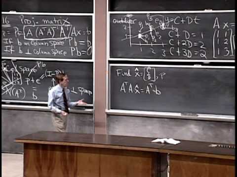 Watch on YouTube →
Overview
Projection matrices split a vector into its closest point in a matrix's column space and a perpendicular error, with the projection given by P = A(AᵀA)⁻¹Aᵀ when A has independent columns. A three-point line-fitting example derives the least-squares normal equations and finds the best line y = 2/3 + t/2; the lecture then proves why AᵀA is invertible and previews orthonormal columns.
Key takeaways
- The projection P = A(AᵀA)⁻¹Aᵀ sends any vector b to its nearest point in the column space of A, provided A has independent columns.
- Least squares minimizes ||Ax − b||²; its minimizer satisfies AᵀA x̂ = Aᵀb, known as the normal equations.
- For the points (1,1), (2,2), and (3,2), least squares gives C = 2/3 and D = 1/2, so the fitted line is y = 2/3 + t/2.
- At the least-squares solution, the residual b − Ax̂ is perpendicular to every column of A and therefore belongs to N(Aᵀ).
- If A has independent columns, xᵀAᵀAx = ||Ax||² proves that AᵀA has no nonzero null vectors and is invertible.
- Orthonormal columns make AᵀA the identity matrix, simplifying the algebra of projections and least-squares solutions.
Chapters
0:00
Projection Matrices Preserve Column-Space Vectors and Eliminate Perpendicular Ones
- For a matrix A with independent columns, P = A(AᵀA)⁻¹Aᵀ projects b onto the column space of A.
- If b is already in the column space, write b = Ax; applying P returns Ax, which equals b.
- If b is perpendicular to every column of A, then Aᵀb = 0 and Pb = 0.
- The complementary projection I − P gives the perpendicular component, and P plus I − P reconstructs the original vector.
8:30
Set Up a Best-Fit Line for Three Inconsistent Data Points
- The data points are (1,1), (2,2), and (3,2), and no single line passes through all three.
- Model the line as y = C + Dt, giving three equations: C + D = 1, C + 2D = 2, and C + 3D = 2.
- Write the system as Ax = b, where A has columns (1,1,1) and (1,2,3), x = (C,D), and b = (1,2,2).
- Because b is not in the column space of A, exact solution is impossible; choose C and D to minimize the error instead.
11:00
Define Least Squares as Minimizing the Sum of Squared Residuals
- The residual vector e = Ax − b records the three vertical differences between observed heights and the fitted line.
- Least squares minimizes the squared length of e, equivalently the sum e₁² + e₂² + e₃².
- The squared-error objective is widely used in regression because it leads to a clean linear system.
- Squaring gives outliers disproportionate influence, so a single unusually large measurement error can substantially change the fitted line.
17:00
Interpret the Fit as the Closest Point in the Column Space
- The fitted values P₁, P₂, and P₃ form a vector in the column space of A, since they are generated by a line C + Dt.
- The least-squares fit selects the point in that column space closest to b = (1,2,2).
- The data plot shows vertical residuals, while the vector-space plot shows b decomposed into its projection and perpendicular error.
- The fitted parameter vector determines the projection through P = Ax̂.
20:00
Derive and Solve the Normal Equations for the Three-Point Fit
- The minimizing parameters satisfy AᵀA x̂ = Aᵀb, the normal equations used in least-squares estimation.
- For the example, AᵀA = [[3,6],[6,14]] and Aᵀb = (5,11), giving 3C + 6D = 5 and 6C + 14D = 11.
- Elimination yields D = 1/2 and C = 2/3, so the best-fit line is y = 2/3 + t/2.
- Setting the partial derivatives of the squared-error function with respect to C and D to zero produces the same normal equations.
24:00
Compute the Fitted Values and Verify Orthogonal Residuals
- Evaluating y = 2/3 + t/2 at t = 1, 2, and 3 gives the fitted vector P = (7/6, 5/3, 13/6).
- Using e = b − P gives e = (−1/6, 1/3, −1/6), and b = P + e.
- The dot product Pᵀe is zero, confirming that the residual is perpendicular to the projection.
- The residual is also perpendicular to both columns of A: (1,1,1) and (1,2,3), so it lies in the null space of Aᵀ.
30:00
Connect Regression Geometry to Projection and Residual Spaces
- The fitted vector P lies in the column space of A, while the residual e lies in its perpendicular complement, N(Aᵀ).
- In the data plot, the residuals are vertical differences; in the vector-space picture, they form one perpendicular error vector.
- The best-fit parameters C and D specify the combination of A's two columns that produces P.
- For line-fitting homework, solve the normal equations for x̂ and then calculate the fitted values with P = Ax̂.
35:50
Prove Independent Columns Make AᵀA Invertible
- To establish invertibility, assume AᵀAx = 0 and show that the only possible x is the zero vector.
- Left-multiplying by xᵀ gives xᵀAᵀAx = (Ax)ᵀ(Ax) = 0, the squared length of Ax.
- A vector with squared length zero must be zero, so Ax = 0.
- Independent columns imply that Ax = 0 has only the solution x = 0; therefore AᵀA has a trivial null space and is invertible.
44:00
Preview Orthonormal Columns and the Identity Gram Matrix
- Perpendicular nonzero columns are independent; requiring each column to have unit length gives an orthonormal set.
- The standard basis vectors in three dimensions are orthonormal, and a matrix formed from them has AᵀA = I.
- In two dimensions, (cos θ, sin θ) and (−sin θ, cos θ) are unit vectors with zero dot product.
- Orthonormal vectors simplify projection calculations and form the starting point for the next lecture's methods for constructing orthonormal bases.
Summary, takeaways, and chapters were generated by AI from the video's transcript and may contain errors. The video belongs to its creator, MIT OpenCourseWare.