Wed Sep 9, 2026 Lecture (L07) Stewart Sect. 2.2 The Derivative as a Function

Overview

The lecture develops the derivative as a function, moving from the instantaneous rate of change at a single input to the difference-quotient function f′(x) = limₕ→₀ [f(x+h) − f(x)]/h. It also uses f(x) = 2/x to show why the Intermediate Value Theorem requires continuity, illustrates estimating derivative values from a graph, and derives f′(x) = 2x − 2 for f(x) = x² − 2x − 3.

Key takeaways

The Intermediate Value Theorem guarantees a root between opposite-sign endpoint values only when the function is continuous across the full closed interval.
For f(x) = 2/x, the endpoint values on [−1, 1] have opposite signs, but the function is undefined at zero; solving 2/c = 0 directly confirms that it has no roots.
The derivative at a fixed input, f′(a), is a numerical tangent slope, while f′(x) is a function assigning tangent slopes across the domain.
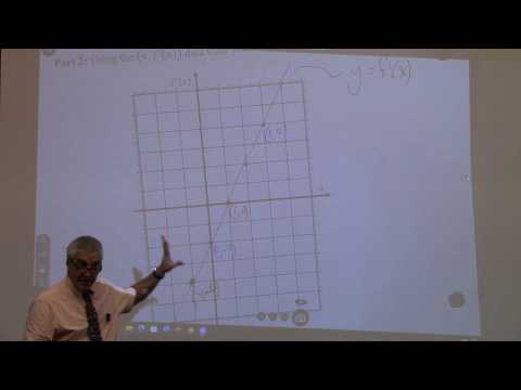
A derivative graph is built by plotting points (x, f′(x)); at x = −1, the lecture estimates a tangent slope of about −4, producing (−1, −4).
Using the limit definition for f(x) = x² − 2x − 3 requires expanding f(x+h), subtracting the entire f(x), factoring and canceling h, then evaluating the limit to obtain 2x − 2.

Chapters

0:00 Friday Quiz Preview and the Root Test for f(x) = 2/x

The Friday quiz includes a problem based on suggested exercises from Stewart section 2.2 and at least one problem similar to a textbook example.
The opening question asks whether f(x) = 2/x has a root on the interval [−1, 1].
A proposed argument uses f(−1) = −2 and f(1) = 2 to claim a root, setting up a check of the Intermediate Value Theorem.

4:32 Using the Intermediate Value Theorem Hypotheses

A root on [−1, 1] would mean finding c in that interval with f(c) = 0; the target output is y = 0.
For f(x) = 2/x, the endpoint values −2 and 2 do bracket zero.
The Intermediate Value Theorem also requires f to be continuous on the entire closed interval [−1, 1].

8:50 Why the Discontinuity at x = 0 Blocks the Theorem

Since 2/x is undefined at x = 0, it is not continuous on [−1, 1].
Opposite signs at the endpoints do not prove a root when the continuity hypothesis fails.
The failure of the theorem’s conditions means it cannot determine whether a root exists; it does not itself prove that no root exists.

12:04 Showing 2/x Has No Roots and Interpreting Its Graph

Solving f(c) = 0 gives 2/c = 0, which is impossible because the numerator is 2, not zero.
The graph passes through (1, 2) and (−1, −2) but never touches the x-axis, so 2/x has no roots.
The graph’s separate positive and negative branches illustrate how a function can change sign without crossing zero when it is discontinuous.

15:23 Why a Valid IVT Proof Must Check Every Condition

A solution invoking the Intermediate Value Theorem must state and verify continuity as well as the endpoint-value condition.
Skipping a hypothesis is not acceptable even when the function happens to be continuous and the conclusion happens to be correct.
The lecture connects this rigor to the earlier quiz problem, described as a textbook example involving a polynomial.

16:44 From Instantaneous Velocity to the Derivative Function

The previous lesson’s average rate of change was the slope of a secant line, computed as a change in output divided by a change in input.
Taking a limit as h approaches zero brings the second point toward the first and gives the tangent-line slope, or instantaneous rate of change.
At a fixed input a, f′(a) is a number; replacing a with the variable x makes f′(x) a function whose values are tangent slopes.

24:19 Estimating f′(−1) from a Graph

To plot a point on the derivative graph at x = −1, estimate the slope of the tangent to the original graph at that input.
The original graph’s point is (−1, 0), but its y-value 0 is not the derivative value.
A hand-estimated tangent drops about 4 units for each 1 unit to the right, giving f′(−1) ≈ −4 and the derivative-graph point (−1, −4).

30:35 Deriving f′(x) = 2x − 2 from the Difference Quotient

For f(x) = x² − 2x − 3, the definition requires building and evaluating limₕ→₀ [f(x+h) − f(x)]/h rather than using a derivative shortcut.
Expanding f(x+h) gives (x+h)² − 2(x+h) − 3; subtracting all of f(x) requires parentheses so the signs distribute correctly.
After cancellation, the numerator is 2xh + h² − 2h; factoring out h and canceling for h ≠ 0 leaves 2x + h − 2.
Substituting h = 0 after cancellation yields the derivative function f′(x) = 2x − 2.

40:23 Matching the Algebraic Derivative to the Graph and Previewing Homework

The formula x² − 2x − 3 describes the original graph, while 2x − 2 describes its derivative graph, connecting the algebraic and graphical methods.
Suggested section 2.2 practice includes #29, finding f′(a) for a square-root function, and #23, finding a derivative function for another square-root expression.
Additional rational-function exercises include section 2.1 #27 and section 2.2 #25; the lecture flags conjugate multiplication and common-denominator algebra as challenges.
The next class is Friday, when the quiz will take place and a difficult derivative problem not covered by a textbook example is scheduled.

Summary, takeaways, and chapters were generated by AI from the video's transcript and may contain errors. The video belongs to its creator, Barsamian's Math Videos.