UUtah Data Mining | Fall 2026 | L8: Hierarchical Agglomerative Clustering

Overview

Clustering groups data points according to a chosen distance or similarity, but what counts as a good grouping depends on the structure being sought: compact blobs, separated groups, or connected shapes. The lecture develops hierarchical agglomerative clustering (HAC) and its single-link, complete-link, average-link, and variance-based choices, then introduces DBSCAN and kernel-density thresholding as ways to find density-connected regions and mark outliers.

Key takeaways

Clustering results depend on the representation and distance function as well as the algorithm; a poor notion of similarity can make otherwise reasonable methods produce unhelpful groups.
Single linkage uses the minimum cross-cluster distance and can recover connected, non-convex shapes such as the two interlocking moons.
Complete linkage uses the maximum cross-cluster distance, favoring groups without very distant members and potentially producing different results from single linkage on the same data.
HAC preserves a nested merge hierarchy, letting users select a cluster count later; a straightforward implementation can cost roughly O(n³), with specialized variants often reducing that cost.
DBSCAN defines clusters as connected components formed from epsilon-neighbor relationships involving core points, and it can leave isolated observations unassigned as outliers.
Kernel-density clustering smooths point neighborhoods with a Gaussian KDE and treats connected regions above a density threshold as clusters.

Chapters

0:00 Clustering Unit: Distances, Algorithms, and Model Choices

The next four lectures cover clustering, beginning with hierarchical agglomerative clustering and then moving to k-means, spectral clustering, and choosing the number of clusters.
A distance or similarity measure is a key input; how raw data is represented can matter more than choosing among familiar vector distances.
When data has obvious groups, many clustering methods may work; when it does not, no algorithm guarantees meaningful clusters.

4:04 Clustering Inputs and the Hard-Partition Output

The input is a dataset X in a metric space, often represented as points in R^d, plus a distance function and commonly a cluster-count parameter K.
Hard clustering returns disjoint subsets S1 through Sk whose union is X, so every point belongs to exactly one cluster.
Some methods relax full coverage and leave distant points unassigned as outliers; soft clustering can also relax disjoint membership.

7:12 Visual Inspection: Plot the Points and Draw the Clusters

For data that can be plotted, visually circling groups is a practical baseline for checking whether clusters make sense.
Two-dimensional plots are especially useful; dimensionality reduction can sometimes create a view for higher-dimensional data, though it should be checked against other results.
The lecture distinguishes partitioning data into groups from other fields’ use of “clustering” to mean detecting unusually dense geographic regions.

17:24 Cluster Quality: Within-Group Width and Between-Group Split

A useful general view of clustering balances width—small distances between points in the same cluster—with split—large distances between points in different clusters.
Possible objectives combine width and split, such as minimizing width relative to split, or may focus only on cluster width.
Different formulations encode different notions of good structure, so results depend on both the chosen objective and the distance measure.

24:10 HAC Algorithm: Repeatedly Merge the Closest Clusters

Hierarchical agglomerative clustering (HAC) initializes every data point as its own cluster.
At each iteration, HAC finds the closest pair of clusters and merges them into their union.
The procedure needs a stopping rule, such as stopping at K clusters or when the closest remaining clusters exceed a distance threshold.

30:03 Cluster Distance Options: Representatives and Pairwise Comparisons

A representative-point approach compares cluster centers; in Euclidean space, the coordinate-wise mean is a common center.
Means are not directly available for objects such as documents unless they have first been embedded in a vector space.
When only point-to-point distances are available, HAC can compare all cross-cluster pairs using rules such as minimum or average distance.

35:08 Single, Average, Variance, and Complete Linkage

Single linkage defines cluster distance as the minimum distance between any cross-cluster point pair.
Average linkage uses the mean of cross-cluster pairwise distances; sampling can estimate it when computing every pair is costly.
A variance-based rule evaluates the spread of the merged cluster, while complete linkage uses the maximum cross-cluster distance.
Complete linkage resists merging clusters that contain even one very distant pair; single linkage instead emphasizes the closest connection.

42:44 Two Moons: Single Linkage Preserves Connected Shapes

On the interlocking two-moons dataset, single linkage can recover each crescent as a cluster by joining locally close neighboring points.
Complete linkage may split a crescent or group points across the moons because distant points within one cluster are penalized.
The example shows why linkage choice should reflect whether the desired structure is connectivity or compact, separated groups.

48:36 Clustering Evaluation Depends on the Desired Structure

Cross-validation comparisons require a cost function, but different clustering linkages encode different costs and therefore different definitions of success.
There is no universal ground-truth ranking between single linkage and compact-cluster methods without specifying the structure sought.
For datasets with clear, separated blobs, many formulations may agree; boundary cases such as two moons expose their differing assumptions.

51:00 HAC Builds a Hierarchy Before Choosing the Cluster Count

With five example points, successive merges can join points 1 and 2, points 4 and 5, and then point 3 with the 1–2 cluster.
The full sequence of merges forms a hierarchy, so users can choose later where to cut it rather than fixing K before clustering.
Hierarchical trees also represent nested groupings, as in phylogenetic trees built from similarities between species’ genomes.

55:49 HAC Runtime: Naive Cubic Cost and Faster Variants

A straightforward implementation may perform up to n merge rounds and repeatedly examine O(n²) cluster pairs, yielding roughly O(n³) work.
Computing some cluster distances, including matching-based distances, can add further cost; specialized variants can reduce runtime to around O(n²) or O(n² log n).
HAC is practical for smaller datasets but can be burdensome at scale, motivating faster density-based alternatives.

1:02:03 DBSCAN Parameters: Epsilon Radius and Minimum Points

DBSCAN uses epsilon to define a neighborhood radius and min points (often written MinPts) to set the density requirement.
A core point has at least MinPts data points within its epsilon-radius neighborhood.
For example, with MinPts set to 3, a point with at least three neighbors in its epsilon ball qualifies as a core point.

1:07:09 DBSCAN Clusters: Core-Point Graphs and Outliers

DBSCAN connects points less than epsilon apart when at least one endpoint is a core point.
Connected components of this graph define clusters; nearby non-core points can join a component through core points.
Points not assigned to any connected component are labeled outliers, and the approach approximates single-link connectivity without building every HAC merge.

1:11:58 Gaussian KDE Clustering: Threshold Density Regions

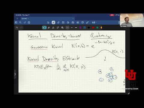
A Gaussian kernel assigns a smooth similarity bump around each point, with a scale parameter sigma controlling its spread.
Kernel density estimation (KDE) averages these bumps over the dataset to estimate density at any query point.
Clusters can be defined as connected regions where KDE exceeds a threshold; points outside those regions are outliers.
KDE thresholding offers smoother boundaries than DBSCAN’s fixed epsilon neighborhoods, though identifying connected regions still requires additional computation.

1:14:00 Choosing a Clustering Formulation for the Data

The lecture closes by emphasizing that clustering has many valid formulations, each designed to reveal particular structure rather than a universal answer.
DBSCAN is a practical density-based option for connected shapes such as two moons, while HAC provides an interpretable merge hierarchy.
The next lecture turns to k-means, described as one of the most widely used clustering approaches.

Summary, takeaways, and chapters were generated by AI from the video's transcript and may contain errors. The video belongs to its creator, UofU Data Science.