UUtah Data Mining | Fall 2026 | L2 - Statistical Phenomenon

Overview

The lecture introduces probabilistic thinking for data mining: data is often modeled as independent, identically distributed (IID) samples, but random variation alone can produce surprising patterns. Using uniform hashing and birthdays, it explains why collisions appear around √m samples, then derives the coupon collector’s mHₘ ≈ m ln m expected samples for seeing every one of m outcomes.

Key takeaways

Under uniform sampling from m possibilities, the first collision becomes likely after roughly √m draws; for 365 birthdays, the 50% threshold is about 23 people.
A hash function can be deterministic for each input while still having probabilistic collision guarantees when analyzed over a randomly chosen salt or hash-function family.
Complete coverage is much more demanding than finding one duplicate: the coupon collector’s expected sample count is mHₘ ≈ m(ln m + 0.577).
A collision, a nearby pair, or an unobserved region can arise from natural random variation and does not by itself establish meaningful structure in a dataset.
Statistical approximations have valid ranges: if n exceeds the number m of possible outcomes, a collision is certain, even though a simplified birthday-probability formula may fail to reflect that.
For randomized algorithms, inspecting plots against expected distributions is a practical correctness check when output variation makes ordinary deterministic tests insufficient.

Chapters

0:00 Course Website, Lecture Materials, and Homework 1

Lecture notes, slides, and recordings are linked from the course website; the notes provide a more formal, overcomplete version of class material.
Homework 1 was posted with an Overleaf template and was scheduled for September 8, with submission through Gradescope.
The assignment focuses on implementing and simulating probabilistic experiments introduced in class.

8:20 Evaluating Probabilistic Code Through Plots

For randomized algorithms, output plots can reveal whether results fall within expected variation even when code review is impractical.
Homework grading will emphasize experiment outputs and plots; readable code may help explain mistakes and earn partial credit.
Students should learn to judge whether a probabilistic result looks plausible rather than relying only on deterministic unit tests.

11:30 IID Samples as a Foundation for Data Analysis

The lecture models a dataset as observations x₁ through xₙ drawn independently and identically from an underlying distribution.
Independence means one observation does not affect another; identical distribution means all observations come from the same source.
IID is a convenient approximation, not a perfect description of changing worlds, sampling without replacement, or data collection that alters future outcomes.

14:00 Sample Size, Estimation, and the Central Limit Theorem

As sample size n grows, estimates generally become more reliable and reflect the underlying distribution more closely.
The Central Limit Theorem provides a foundation for understanding how sample-based quantities behave as n increases.
A central data-science question is how many samples are needed for a desired accuracy—or how much to trust analysis of a fixed dataset.

17:10 Uniform Samples from a Finite Universe

The lecture represents each observation as an element of a discrete universe of size m, indexed from 0 to m−1.
Example universe sizes include roughly 10¹⁶ IP addresses, about 100,000 language-model tokens, and hundreds of millions or billions of people.
The baseline distribution assigns probability 1/m to each possible value, providing a model with no unusually popular outcomes or other special structure.

21:10 Hash Tables, Uniform Hashing, and Random Salts

A simple set representation uses an array with a 0 or 1 at each position; a hash function maps an input, such as a word or file, to an array index.
A uniform hash aims to make distinct items collide with probability 1/m, while remaining deterministic for a fixed input and hash configuration.
A randomly selected salt or seed changes the hash mapping; after it is fixed, hashing remains deterministic, and SHA-1 is mentioned as a familiar hash-function example.

27:12 Birthday Paradox Demonstration: A Collision After 38 People

The class treats birthdays as draws from a universe of 365 days and records dates until two people share one.
A collision appeared after 38 reported birthdays, well before collecting birthdays from all 365 possible days.
The key observation is that a match can be between any pair; no particular birthday needs to be selected in advance.

34:00 Birthday Collision Probability and Pair Counting

With two people, the collision probability is 1/365; with n people, there are n choose 2 possible pairs to compare.
A rough approximation for collision probability is 1 − (1 − 1/m)^(n choose 2), although pairwise collision events are dependent and the expression is not exact.
For m = 365, the approximate probability reaches about 50% around 23 people; the lecture’s rough estimate for 38 people is about 88%.

44:10 Why Hash Collisions Begin Around √m Samples

The birthday calculation gives the central scaling rule: a collision becomes likely after roughly √m samples, not after m samples.
For a hash array with 20,000 slots, √m is about 141, so collisions can begin after only a few hundred inserted items.
Hash-table implementations therefore need collision-handling strategies even when hash outputs are intended to be uniform.

49:00 Birthday-Model Assumptions and Where Approximations Fail

Human birthdays are close to uniform, but seasonality, leap-day birthdays, twins, or selection effects—such as age cutoffs in hockey—can change collision rates.
The simplified probability expression is useful for moderate n but cannot be a valid exact model for every range; if n exceeds m, a collision is guaranteed by the pigeonhole principle.
Data scientists should match approximations to the parameter range and distinguish model errors from ordinary random variation.

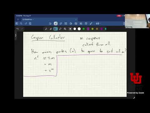
1:01:10 Coupon Collector: How Many Draws to See Every Outcome?

The coupon collector problem asks how many independent uniform draws are needed to observe all m distinct outcomes.
Examples include collecting every toy in cereal boxes, every Happy Meal toy, or every desired Pokémon from packs.
The target is complete coverage, which is different from the birthday problem’s goal of finding just one repeated outcome.

1:06:30 Breaking Complete Coverage into New-Item Waiting Times

Let Tᵢ count the draws needed to move from i−1 distinct outcomes to i distinct outcomes; total collection time is the sum of these waiting times.
When i−1 outcomes have been seen, the chance that the next draw is new is (m−i+1)/m.
The expected waiting time for that next new outcome is therefore m/(m−i+1), making the stages easy to add.

1:09:40 Harmonic Numbers Give the Coupon Collector Expectation

Summing the stage expectations gives E[T] = m(1 + 1/2 + … + 1/m) = mHₘ.
The harmonic number satisfies Hₘ ≈ ln m + γ, where γ, the Euler–Mascheroni constant, is approximately 0.577.
Thus the expected number of draws is approximately m(ln m + 0.577), or order m log m.

1:12:00 Why the Final Coupon Makes Collection Take m log m

The first half of the distinct outcomes are found relatively quickly, but the chance of drawing a new outcome falls as the collection fills.
Near completion, the final missing outcome takes about m draws on average; the second-to-last takes about m/2, and earlier late-stage waits also grow.
This long tail explains why complete collection takes substantially more than the intuitive m draws, even under a uniform distribution.

1:15:40 Use Collision and Coverage Baselines to Interpret Data

A collision around √m samples can be ordinary random behavior, while observing every one of m outcomes generally takes roughly m ln m samples.
For m = 20,000, full coverage can require on the order of hundreds of thousands of draws, rather than just 20,000.
Homework 1 asks students to simulate the birthday and coupon-collector experiments across different n and m values and compare plots with theoretical expectations.

Summary, takeaways, and chapters were generated by AI from the video's transcript and may contain errors. The video belongs to its creator, UofU Data Science.