UUtah Data Mining | Fall 2026 | L10: Spectral Clustering

Overview

Spectral clustering turns a graph or similarity matrix into a clustering by constructing a graph Laplacian, computing its eigenvectors, and using the low-eigenvalue coordinates to divide or recluster vertices. The lecture motivates normalized cuts as a balance-aware alternative to minimum cuts, explains the Fiedler vector and normalized Laplacian, and shows how spectral embeddings can feed threshold sweeps or K-means; it also covers homework and project-report expectations.

Key takeaways

Minimum edge cut can isolate a low-degree vertex and produce a poor partition; normalized cut adds volume terms to favor more balanced graph splits.
For a connected graph, the unnormalized Laplacian L₀ = D − A has a constant first eigenvector, while the second-smallest-eigenvalue eigenvector—the Fiedler vector—provides a useful one-dimensional partition coordinate.
Thresholding the Fiedler vector at zero is a convenient starting point, but sorting its coordinates and sweeping possible thresholds can find a better normalized cut.
Spectral embeddings can support more than binary partitions: retain multiple eigenvector coordinates, scale by inverse eigenvalues, and apply K-means to identify several clusters.
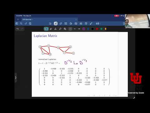
The normalized Laplacian, D⁻¹ᐟ²(D − A)D⁻¹ᐟ², is preferred here for practical clustering; replacing binary adjacency with weighted similarities extends the method to affinity graphs.
Sparse matrix representations store only graph edges and are essential when a graph has far fewer than n² edges, while still enabling many linear-algebra operations.

Chapters

0:00 Spectral Clustering Preview and Course Announcements

Spectral clustering uses eigenvalue decompositions to find clusters and also provides a form of nonlinear dimensionality reduction.
The lecture previews graph and matrix representations, which will connect clustering to later linear-algebra topics.

2:00 Homework 3: Comparing Clustering Algorithms

Homework 3 covers hierarchical clustering and assignment-based methods, including Gonzalez, k-means, and k-means++.
The randomized k-means++ portion should be run at least 20 times; comparing cumulative cost distributions reveals that results vary between trials.
One dataset contains 50-dimensional word vectors, so plotting alone will not identify its cluster structure.

5:50 Data Collection Report and Simulation Planning

One person per project group submits a one-page report answering five questions about the dataset, due the following Tuesday.
Describe the data’s dimensions and representation—such as vectors, sets, matrices, or graphs—rather than just its file size or CSV format.
Propose how to simulate proxy data, especially when real data is private or restricted; a useful simulation can establish a baseline or encode expected clusters.

12:00 Spectral Clustering as a Top-Down Graph Method

The clustering input can be a graph or similarities rather than only points and pairwise distances.
Unlike bottom-up agglomerative clustering, spectral clustering repeatedly splits vertex sets and can stop after only a few levels.
A graph can be derived from point distances, for example with a k-nearest-neighbor graph.

14:00 Where Spectral Clustering Fits Among Clustering Methods

Agglomerative hierarchical clustering merges nearby clusters from the bottom up; density-based methods can provide a shortcut to some hierarchical results.
Assignment-based clustering, exemplified by k-means, assigns each data point to its nearest site.
Spectral clustering instead focuses on splitting a graph into two parts, then recursively splitting the resulting vertex subsets if needed.

19:00 Graph Vertices, Edges, and the Adjacency Matrix

Graph vertices represent the data points to be clustered, while edges encode relationships that stand in for distances or similarities.
For an undirected graph, the adjacency matrix is symmetric: an entry is 1 for an edge and 0 otherwise.
With no self-loops, the adjacency matrix diagonal is zero; the same edge appears in both mirrored matrix entries.

27:00 Sparse Graph Storage at Scale

Many large graphs have only tens or hundreds of edges per vertex, far fewer than the possible n² vertex pairs.
A dense adjacency matrix requires n² entries, while sparse matrix formats store only nonzero entries, such as neighbor lists.
Sparse linear-algebra libraries can perform operations such as matrix multiplication without materializing all the zeros.

30:10 Why Minimum Edge Cuts Can Produce Bad Clusters

A cut partitions vertices into S and T, and its size counts the edges crossing between the two sets.
A minimum cut may isolate a low-degree vertex such as H by removing only one edge, producing an undesirable, highly unbalanced cluster.
The graph example also admits a one-edge cut between larger groups, showing that cut size alone does not express cluster quality.

37:00 Normalized Cut Balances Separation and Cluster Volume

The volume of a vertex set counts edges with at least one endpoint in that set, including crossing edges.
Normalized cut scores a partition as cut(S,T)/vol(S) + cut(S,T)/vol(T), penalizing cuts that isolate small, low-volume groups.
In the example, isolating H scores 1.1, while the more balanced split has a normalized-cut score of about 0.367.

44:00 Recursive Normalized-Cut Clustering and the Graph Laplacian

The top-down procedure finds a low-normalized-cut partition, keeps each side’s induced edges, and can recurse on each side.
The unnormalized Laplacian is L₀ = D − A, where A is the adjacency matrix and D is the diagonal matrix of vertex degrees.
Each Laplacian row and column sums to zero because the degree on the diagonal balances the negative adjacency entries.

52:00 Laplacian Eigenvectors and the Fiedler Vector

For a symmetric Laplacian, the eigendecomposition expresses the matrix using orthogonal eigenvectors and a diagonal matrix of eigenvalues.
The first eigenvector of a connected graph is constant and carries little partition information; the second, associated with the second-smallest eigenvalue, is the Fiedler vector.
Each Fiedler-vector coordinate maps one graph vertex into one dimension, giving a signal for separating vertices.

1:00:00 Using the Fiedler Vector to Split a Graph

Thresholding Fiedler-vector coordinates at zero can recover a useful normalized-cut partition in the illustrated graph.
Zero is not always the best threshold: sorting the coordinates and sweeping candidate split points can search for a lower normalized cut.
A gap between sorted coordinates can indicate a natural place to divide the graph.

1:03:00 Spectral Embeddings, Random Walks, and Eigenvalue Ordering

The embedding aims to place vertices with strong graph connectivity near one another, reflecting where a random walk is likely to travel.
For the Laplacian, eigenvalues are considered in increasing order; the second-smallest eigenvalue and its vector provide the leading nontrivial partition signal.
Additional eigenvectors contribute further orthogonal structure, allowing a graph to be represented in more than one dimension.

1:08:00 Graph Symmetry, Multidimensional Embeddings, and K-Means

Vertices A and D have identical neighborhoods in the example, so their Laplacian-embedding coordinates match and the graph representation cannot distinguish them.
Using multiple eigenvector coordinates can expose several groups, including the example’s isolated C and H alongside larger vertex groups.
A common workflow scales embedding coordinates by inverse eigenvalues, retains useful dimensions, and runs Lloyd’s K-means algorithm, potentially with k-means++ initialization.

1:15:00 Affinity Matrices and the Normalized Laplacian

A weighted affinity matrix replaces binary adjacency entries with pairwise similarities; each vertex’s degree becomes the sum of its affinity weights.
The normalized Laplacian is L = D⁻¹ᐟ²(D − A)D⁻¹ᐟ², equivalently I − D⁻¹ᐟ²AD⁻¹ᐟ².
The lecture recommends the normalized Laplacian for practical spectral clustering, using its eigenvectors for recursive splits, threshold sweeps, or a lower-dimensional K-means step.

1:20:00 Spectral Clustering Options and Choosing K Next

Practical options include thresholding the second eigenvector, sweeping for a better cut, or clustering a multidimensional spectral embedding.
The same workflow accepts graphs or similarity functions represented as affinity matrices.
The next lecture will address how to choose the number of clusters, K.

Summary, takeaways, and chapters were generated by AI from the video's transcript and may contain errors. The video belongs to its creator, UofU Data Science.