UUtah Data Mining | Fall 2026 | Choosing k (#clusters)

Overview

Choosing the number of clusters has no universally correct answer: the best method depends on the data, distance measure, clustering objective, and desired level of detail. The lecture compares visual inspection, the elbow method, silhouette scores, and Bayesian Information Criterion (BIC), emphasizing that plots and automated scores need human judgment and that some data may not have meaningful clusters at all.

Key takeaways

For k-means-style costs, increasing K can only reduce or preserve the clustering cost, and K equal to the number of points can drive squared-error cost to zero; choose an elbow rather than the minimum.
A two-dimensional plot is a valuable first check, but PCA, multidimensional scaling, or spectral embeddings can hide structure when projection loses information.
A dense clump with a long sparse tail may have no natural cluster count; changing features or applying a log transform can change the distance geometry, and declining to cluster may be the sound conclusion.
Silhouette scoring compares each point’s average within-cluster distance a with its best alternative-cluster distance b using (b − a) / max(a, b); it favors K values where points fit their assigned groups better than alternatives.
A dataset with 11 small groups nested inside three larger groups can support both K = 11 and K = 3; the useful choice depends on whether the task needs fine or broad segments.
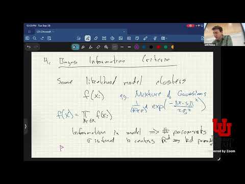
BIC selects K by minimizing −2 log-likelihood plus a parameter-count penalty, but its formal recommendation depends on trusting the likelihood model used to describe the clusters.

Chapters

0:00 Course Logistics: Clustering Assignment, Streaming Data, and the Midterm

The lecture finishes the clustering unit; the next topic is streaming data that arrives too quickly or in too large a volume to store.
Clustering Assignment 3 covers hierarchical clustering, assignment-based clustering, and choosing the number of clusters; it is due the following week.
The midterm will cover material through clustering, exclude streaming, and allow one double-sided reference sheet or two single-sided sheets.

3:04 Data Collection Reports: Representing Data and Planning Simulations

The data collection report should be at most one page per group and explain how collected data will become vectors, sets, matrices, or graphs for analysis.
Groups should describe challenges in collecting or representing their data and propose how they might simulate similar data.
A redistricting research example uses roughly 30 survey responses describing preferred district shapes as a starting point for generating more data.

8:58 Synthetic Data as a Baseline, Not a Substitute for Real Data

Simulations can help estimate how runtime and noise change as a dataset grows, but they may not reflect the structure of the actual data.
With only 50 observations and an assumed six-cluster structure, a sample may not display cleanly separated clusters.
Treat simulated results as a comparison baseline; investigate why real-data results differ rather than assuming the simulation is authoritative.

13:39 Midterm Format and How to Practice for It

The 80-minute midterm is closed-book and closed-computer, with a permitted reference sheet and no calculator; calculations should be simple.
The linked practice test reflects question style and difficulty but emphasizes some older topics, including k-grams, Jaccard similarity, and minhashing.
To create additional practice, provide an AI tool with the course topics and notes and ask it to generate structurally similar questions.

21:00 Four Approaches to Choosing the Number of Clusters

The lecture introduces visual inspection, the elbow method, silhouette scores, and Bayesian Information Criterion (BIC).
Visual inspection and the elbow method require less modeling; silhouette scoring assumes mean-like clusters, while BIC requires a likelihood model.
Trying multiple approaches is useful because each method has assumptions and may give a different answer.

25:29 Visual Inspection: Four Separated Blobs Make K = 4 Clear

When two-dimensional data shows four distinct groups, plotting it makes K = 4 an evident choice.
A plot can also expose an isolated point that may be an outlier rather than a fifth cluster.
When the data can be plotted directly, visual inspection is a strong first check and keeps a human involved in the decision.

27:14 Projecting High-Dimensional Data for Cluster Inspection

For data with more than two dimensions, dimensionality reduction can produce a view for inspection, including PCA, multidimensional scaling, and spectral methods.
A spectral embedding can use a similarity or affinity matrix, a normalized graph Laplacian, and leading eigenvectors to create a lower-dimensional representation.
Projection can lose information or overlap groups, so visible clusters are useful evidence but may not reveal every cluster in the original space.

30:05 The “Smear” Problem: When Data May Not Be Clusterable

Real project data may look like a dense clump with points spread outward rather than clearly separated blobs; the lecture calls this a “smear.”
For a smear, K = 1, K = 2, or a larger value such as K = 10 may each serve a different purpose, such as separating density levels or segmenting regions.
A log transform or revised feature representation can change distances and reveal structure, but if no defensible structure appears, deciding not to cluster is reasonable.

36:58 Elbow Method: Compare Clustering Cost Across Values of K

Run a chosen clustering method for multiple values of K and plot its cost, such as the sum of squared distances to assigned centers used by k-means.
As K increases, the best achievable cost cannot increase; with k-means, K equal to the number of data points can reduce the cost to zero.
Because simply choosing the lowest cost would favor excessive clusters, the elbow method looks for where additional clusters bring diminishing returns.

41:43 Reading the Elbow: Diminishing Returns and Human Judgment

Choose a K near the bend where the cost curve begins to flatten; the bend may span several values, making an answer off by one or two clusters plausible.
A gradual, nearly straight cost curve suggests little evidence for a natural cluster count under the chosen cost function.
The elbow approach can help in high dimensions, but it remains a visual judgment and can be applied to other decreasing costs with suitable care.

50:25 Silhouette Score: A Mean-Based Measure with Assumptions

Silhouette scoring assigns each candidate K a score and chooses the K with the maximum average score.
It is most appropriate for mean-like, compact clusters; it may not suit single-link hierarchical clustering or some spectral-clustering results in their original metric.
Its assumptions should match the clustering representation and distance measure rather than being applied automatically to every method.

53:01 Silhouette Formula: Within-Cluster and Replacement Distances

For each point, a is its average distance to the other points in its assigned cluster.
For each point, b is the smallest average distance to the points in any other cluster—the best alternative cluster.
The point score is (b − a) / max(a, b), ranging from −1 to 1; averaging point scores gives the clustering’s overall silhouette score.

1:00:33 Silhouette Example: Why K = 3 Can Beat K = 2 or K = 4

With three well-separated groups, points tend to have short within-cluster distances and larger distances to their best alternative, yielding a relatively high silhouette score.
At K = 4, splitting a natural group can make its points nearly as close to the replacement cluster as to their assigned cluster, lowering their scores.
At K = 2, merging two groups increases within-cluster distances for affected points, also reducing the average score; the maximum can therefore favor K = 3.

1:08:15 Multiple Valid Scales: K = 3 and K = 11 Can Both Be Useful

A dataset may contain 11 small groups arranged into three larger groups, making both K = 11 and K = 3 defensible descriptions.
Silhouette scores may have multiple local peaks, while an elbow curve may flatten near K = 3 and again near K = 11.
Choose the resolution based on the task: three broad population groups and 11 finer segments answer different questions.

1:14:43 BIC: Trade Off Likelihood Fit Against Model Complexity

BIC requires a likelihood model for how clusters generate data; a mixture of Gaussians is one example, assigning points probabilistically to component distributions.
The criterion is BIC = −2 log-likelihood + m log(n), where m is the number of model parameters and n is the number of observations; select the K that minimizes it.
For a center-based model in d dimensions with fixed variance, the lecture illustrates m as K × d; adding clusters can improve fit while increasing the complexity penalty.

1:21:07 Choosing K Is a Judgment Call, Not a Universal Rule

The closing guidance is to combine the available tools and keep a person involved when deciding whether apparent structure is meaningful.
BIC is most suitable when a credible likelihood model is available; simpler plots and elbow curves still require interpretation.
The class will move on to streaming data in the next lecture, and students should submit the data collection report.

Summary, takeaways, and chapters were generated by AI from the video's transcript and may contain errors. The video belongs to its creator, UofU Data Science.