Stanford CS229 Machine Learning | Spring 2026 | Lecture 18: GMM (EM), PCA

Overview

This lecture introduces reinforcement learning (RL) as sequential decision-making without direct supervision, relying instead on rewards. It defines the Markov Decision Process (MDP) framework, comprising states (S), actions (A), transition dynamics (P), rewards (R), and discount factor (gamma), using a 1D robot navigation example. The core goal is to find an optimal policy (pi*) that maximizes expected cumulative reward, often by solving the Bellman equation. The lecture then details the Policy Gradient (REINFORCE) algorithm, a method for optimizing parameterized stochastic policies (pi_theta) by estimating the gradient of the expected return using sampled trajectories.

Key takeaways

Reinforcement Learning (RL) tackles sequential decision-making problems where agents learn from rewards rather than explicit labels, using the Markov Decision Process (MDP) framework.
An MDP is defined by states, actions, transition dynamics, rewards, and a discount factor, with the goal of finding an optimal policy (pi*) to maximize cumulative reward.
The Bellman equation provides a recursive method to calculate value functions, which represent the expected future reward from a given state under a specific policy.
Policy Gradient methods, like REINFORCE, directly optimize a parameterized policy (e.g., a neural network) by estimating the gradient of the expected return.
The log-derivative trick is crucial for estimating policy gradients, allowing computation even when the objective function's dependency on parameters is only through the sampling distribution.

Chapters

0:00 Introduction to Reinforcement Learning and its Applications

Reinforcement Learning (RL) focuses on sequential decision-making, distinct from supervised learning.
Robotics is used as a primary example for understanding RL basics.
The core algorithm introduced is Policy Gradient, applicable to robotics and LLMs.

1:59 Defining Sequential Decision Making

Decision-making involves actions with future ramifications, unlike simple predictions.
Sequential decision-making involves multiple rounds of actions and evaluations.
Greedy algorithms are insufficient due to long-term consequences and the need to balance return vs. risk.

5:34 Exploration vs. Exploitation Trade-off

Exploration involves collecting information for future better decisions, while exploitation maximizes current known rewards.
Many modern applications, especially LLMs, have subtle exploration-exploitation trade-offs, often with limited explicit exploration.
Focus is primarily on managing long-term ramifications of decisions.

7:23 RL's Lack of Supervision and Reliance on Rewards

RL typically operates with little to no direct supervision, unlike classification.
Learning occurs through scalar rewards indicating good/bad actions, not optimal action labels.
Data is collected actively through trial and error.

10:50 The Markov Decision Process (MDP) Framework

MDP is the modeling framework for sequential decision-making and interaction with an environment.
It describes how decisions affect the environment and future states.

13:18 MDP Component: States (S)

States represent all necessary information to describe the world at a given time.
Examples include robot position on a 1D tape, joint angles, or camera images.
The state space (S) can be discrete or continuous, finite or infinite.

18:35 MDP Component: Actions (A)

Actions are the set of possible operations an agent can perform.
Examples include moving left/right for a robot, applying force to joints, or placing a stone on a Go board.

19:58 MDP Component: Transition Dynamics (P)

Transition dynamics (P(S'|S, A)) define the probability distribution over the next state (S') given the current state (S) and action (A).
These dynamics can be deterministic or stochastic.
Example: Moving left from state 7 has a 0.9 chance of reaching state 6 and a 0.1 chance of staying at state 7.

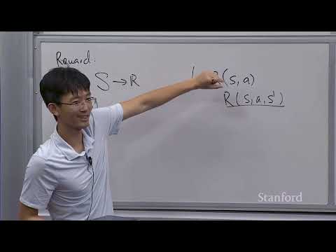
30:12 MDP Component: Reward Function (R)

The reward function R(S) or R(S, A) or R(S, A, S') assigns a scalar value indicating the desirability of a state or state-action pair.
It defines the goal, e.g., reward of 1 for reaching goal state 9, -0.1 for any other state.
Reward shaping can be used to provide intermediate rewards but risks misguiding the agent.

41:49 Defining Return/Payoff for a Trajectory

The total return (or payoff) for a trajectory is the sum of rewards over all steps.
A discount factor (gamma, 0 < gamma <= 1) is often introduced to weigh future rewards less than immediate ones.
Discounting bounds the total payoff and encourages shorter paths.

48:59 The Complete MDP Tuple

An MDP is formally defined by the tuple (S, A, P, R, gamma).
The goal is to find a policy that maximizes the expected return.

53:48 The Markov Property and Policies

The Markov property states that the future state depends only on the current state and action, not the past history.
This implies the optimal action at time t depends only on the current state St.
A policy (pi) is a mapping from states to actions (S -> A), defining the agent's behavior.

1:06:43 Value Functions: V(S) and V*(S)

The value function V_pi(S) estimates the expected total return starting from state S and following policy pi.
V*(S) represents the maximum possible expected return from state S, achievable by an optimal policy pi*.
The optimal policy pi* is the one that maximizes V_pi(S) for all S.

1:12:23 The Bellman Equation

The Bellman equation provides a recursive relationship for value functions, enabling their computation.
For V_pi(S), it relates the value of a state to the immediate reward and the discounted expected value of future states.
It forms a linear system of equations that can be solved for V_pi values.

Summary, takeaways, and chapters were generated by AI from the video's transcript and may contain errors. The video belongs to its creator, Stanford Online.