Stanford AA203 Optimal and Learning-Based Control | Spring 2026 | Lecture 9: Stochastic Dyn. Program

Overview

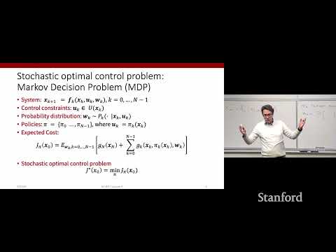
This lecture introduces Markov Decision Processes (MDPs) as a framework for optimal control under uncertainty, extending dynamic programming to discrete-time stochastic systems. Key concepts include state transitions affected by disturbances (WK), control constraints, and optimizing expected costs. The lecture details the dynamic programming recursion for finite-horizon MDPs, illustrating with an inventory control example, and then discusses infinite-horizon MDPs, stationary policies, and the Bellman equation for value functions and Q-functions, setting the stage for reinforcement learning.

Key takeaways

Markov Decision Processes (MDPs) extend dynamic programming to systems with stochastic disturbances, where the probability distribution of disturbances depends only on the current state and control.
In stochastic optimal control, the objective is to find a policy that optimizes the expected cost or reward over all possible realizations of disturbances.
The dynamic programming algorithm for finite-horizon MDPs recursively computes optimal costs-to-go by taking expectations over disturbances at each stage.
For infinite-horizon MDPs, the problem becomes stationary, and the Bellman equation transforms into a fixed-point equation, allowing for stationary optimal policies.
Q-functions, representing the expected cumulative reward from a state-action pair followed by an optimal policy, are crucial for learning-based control when model parameters are unknown.
The stochastic LQR problem shows that even with Gaussian noise, the optimal policy remains linear feedback, with the cost increasing due to the noise magnitude.

Chapters

0:05 Introduction to Stochastic Dynamic Programming and MDPs

Extends optimal control to discrete-time systems with uncertainty.
Introduces Markov Decision Processes (MDPs) for modeling disturbances.
State transition: SK+1 = F(SK, UK, WK), where WK is a disturbance.

0:25 Modeling Disturbances and Probability Distributions

Disturbances (WK) are modeled as random variables.
Probability distribution of WK can depend on current state (SK) and control (UK).
Crucial assumption: WK's distribution does not depend on past states or controls (Markov property).

0:55 Cost Formulation in Stochastic Settings

Stage-wise costs can depend on disturbances (WK).
Costs become random variables due to disturbance dependency.
Optimality is defined by minimizing the expected cost over all disturbance realizations.

2:15 Key Assumptions and Problem Structure

Discrete-time, Markovian model where history is captured by the current state.
Goal: find a closed-loop policy mapping states to optimal control actions.
Additive cost structure and risk-neutral formulation (expectation-based).

5:43 Principle of Optimality in Stochastic Settings

The principle of optimality holds for stochastic dynamic programming.
An optimal policy for the overall problem implies optimal policies for tail subproblems.
Proof is more involved than in deterministic settings, referencing Dimitri Bertsekas.

9:51 Dynamic Programming Algorithm for Finite Horizon MDPs

Algorithm proceeds backward from the terminal stage (N).
Recursively computes the optimal cost-to-go (JK(XK)).
Key difference: expectation over disturbance WK is taken at each step.

23:40 Inventory Control Example: Problem Formulation

State (SK): stock available; Control (UK): purchased stock; Disturbance (WK): demand.
State transition: SK+1 = max(0, SK + UK - WK).
Warehouse capacity constraint: SK + UK <= 2.

26:54 Inventory Control Example: Cost and Disturbances

Demand (WK) distribution: 10% (0 units), 70% (1 unit), 20% (2 units).
Terminal cost = 0.
Stage-wise cost: UK (purchase cost) + (SK + UK - WK)^2 (penalty for surplus/shortage).

33:20 Inventory Control Example: Solving with Dynamic Programming

Terminal cost J3(X3) = 0.
Bellman equation for J2(X2) involves minimizing over U2, considering expected cost over W2.
Manual calculation of J2(0) demonstrates unrolling expectations and finding optimal U2.

40:23 Inventory Control Example: Optimal Policy and Results

Optimal U2 for J2(0) is found to be 1.
Spreadsheet provides results for all stages and states.
Optimal policy is derived for all states and stages, providing a complete control strategy.

45:09 Stochastic Linear Quadratic Regulator (LQR)

LQR with stochastic dynamics: SK+1 = A*SK + B*UK + Wk.
Disturbance Wk is Gaussian with zero mean and covariance Sigma.
Cost function is quadratic: J(X, U) = X'QX + U'RU.

48:29 Solving Stochastic LQR with Dynamic Programming

Assumes cost-to-go is quadratic: JK(XK) = XK'PKXK + CK.
Bellman equation involves expectation over Wk.
Expectation of Wk'PK+1Wk = trace(PK+1 * Sigma).

53:29 Stochastic LQR Solution and Implications

The optimal control policy remains linear feedback, same as deterministic LQR.
The optimal cost increases by a constant term related to noise magnitude.
This demonstrates that dynamic programming can handle stochasticity in LQR.

56:40 Infinite Horizon Markov Decision Processes (MDPs)

Extends finite horizon problems to an infinite number of stages.
Assumes stationary dynamics (transition probabilities independent of time).
Introduces a discount factor (gamma) to manage infinite sums of rewards.

58:51 Infinite Horizon Bellman Equation and Stationary Policies

Optimal policy becomes stationary (independent of time stage).
The Bellman equation becomes a fixed-point equation: V*(X) = max_U [R(X,U) + gamma * E[V*(X')]].
Value iteration and policy iteration are algorithms to solve this equation.

1:10:00 Q-Functions and Their Role

Q-function Q*(X,U) = R(X,U) + gamma * E[V*(X')].
Represents cumulative reward from state X, action U, and optimal policy thereafter.
Q-functions satisfy a fixed-point equation similar to the Bellman equation.

1:11:40 Q-Functions for Learning and Action Selection

Useful when model parameters (like transition probabilities T) are unknown.
Learning algorithms can approximate Q-functions.
Optimal action from state X is the U that maximizes Q*(X,U).

1:13:20 Policy Evaluation for a Given Policy

Value for a fixed policy pi, Q_pi(X,U), can be computed.
This involves solving a linear system of equations if the state space is finite.
Next lecture will cover value iteration and policy iteration algorithms.

Summary, takeaways, and chapters were generated by AI from the video's transcript and may contain errors. The video belongs to its creator, Stanford Online.