Stanford AA203 Optimal and Learning-Based Control | Spring 2026 | Lecture 7: Dynamic Programming

Overview

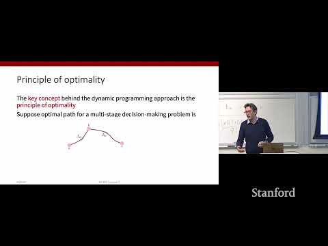
Stanford Online's Lecture 7 on Dynamic Programming introduces closed-loop optimal control policies, contrasting them with open-loop methods. The lecture details the principle of optimality, which states that the tail of an optimal policy is also optimal for the truncated problem. This principle underpins dynamic programming, an algorithm that solves optimal control problems backward in time, demonstrating its application through a shortest path example and the Linear Quadratic Regulator (LQR) problem, which simplifies to recursive matrix equations (Riccati equations).

Key takeaways

Closed-loop optimal control policies, computed via dynamic programming, offer robustness to disturbances by mapping states to optimal actions.
The principle of optimality is the core concept enabling dynamic programming, stating that optimal substructures exist within optimal solutions.
Dynamic programming solves problems backward in time, starting from a known terminal condition, and recursively computes optimal actions and costs.
The 'curse of dimensionality' is a major challenge for dynamic programming, as computational complexity grows exponentially with the state space dimension.
The Linear Quadratic Regulator (LQR) problem, with linear dynamics and quadratic costs, simplifies dynamic programming into recursive matrix equations (Riccati equations).
LQR yields an optimal control law that is a linear feedback of the state (u = -Fx), making it computationally efficient and widely applicable.

Chapters

0:00 Recap of Open-Loop Optimal Control Methods

Reviewed indirect and direct methods for solving optimal control problems in open-loop form.
Indirect methods derive necessary optimality conditions, leading to two-point boundary value problems.
Direct methods discretize the problem into a nonlinear optimization problem.
Direct methods are currently more popular, especially in robotics, due to algorithmic and hardware advances.

5:19 Introduction to Closed-Loop Optimal Control Policies

Shifting focus to methods for closed-loop optimal control.
Goal: find a control law mapping states to optimal controls, not just a time-indexed sequence.
Closed-loop policies are more robust to disturbances and model mismatches.

10:44 Introducing Dynamic Programming for Closed-Loop Control

Dynamic programming is presented as a procedural algorithm for solving optimal closed-loop control policies.
It is computationally more intensive than open-loop methods but yields more powerful, robust policies.
The plan is to derive the algorithm first in discrete time, then extend to continuous time.

13:20 Discrete-Time Optimal Control Problem Formulation

Time is discretized into stages (tk or stage k).
Dynamics are represented by discrete-time update equations (e.g., via Euler discretization).
Control constraints (U) and additive cost functions (stage-wise cost + terminal cost) are defined.

20:26 Objective: Finding Optimal Closed-Loop Policies

The goal is to find an optimal closed-loop policy 'pi' that maps state and time to the optimal control.
This contrasts with open-loop, which optimizes a sequence of controls.
This shift has deep implications for control design and robustness.

22:21 The Principle of Optimality

The key to solving for optimal closed-loop policies lies in the problem's structure, specifically the principle of optimality.
This principle arises from the additive cost function.
It states that an optimal policy's details are optimal for any truncated subproblem.

24:08 Formal Statement and Proof of the Principle of Optimality

The principle states that if a path from A to E is optimal, then the segment from an intermediate point B to E must also be optimal for the problem starting at B.
Proof by contradiction: assuming a non-optimal tail path exists would imply a better overall path from A to E, contradicting the initial assumption.

37:05 Principle of Optimality in Discrete-Time Optimal Control

If u0*, u1*, ..., uN-1* is an optimal control sequence, then the sequence starting from uk* at state xk* is optimal for the subproblem from time k onwards.
Mnemonic: 'The tail of optimal sequences are optimal for the tail subproblems.'

40:41 Intuition: Reusing Computations with the Principle of Optimality

The principle allows reusing pre-computed optimal solutions for tail subproblems.
Instead of brute-forcing all control combinations, one can concatenate immediate decisions with known optimal tail solutions.
This significantly reduces computation by avoiding redundant calculations.

51:44 Dynamic Programming: Solving Backward in Time

Since an oracle for tail problems is unavailable, dynamic programming is used.
The algorithm solves the problem backward in time, starting from the terminal condition where the optimal solution is obvious.
This recursive process builds the optimal policy step-by-step.

54:01 Shortest Path Example of Dynamic Programming

A concrete shortest path problem from 'a' to 'h' is used to illustrate the backward computation.
Costs to reach 'h' from intermediate nodes (g, f, e, d, c, b) are calculated recursively.
The optimal path is found by concatenating immediate costs with pre-computed 'costs to go'.

1:07:21 Challenges and Formalism of Dynamic Programming

Problems must be mapped to the discrete-time, additive-cost formalism.
The algorithm requires computation for all possible states at each time step, leading to the 'curse of dimensionality' (exponential scaling with state dimension).
Approximate dynamic programming is needed for high-dimensional or continuous state spaces.

Summary, takeaways, and chapters were generated by AI from the video's transcript and may contain errors. The video belongs to its creator, Stanford Online.