Stanford AA203 Optimal and Learning-Based Control | Spring 2026 | Lecture 6: Direct Methods

Overview

Stanford Online's Lecture 6 on Direct Methods for Optimal Control introduces techniques to solve optimal control problems by discretizing them into nonlinear optimization problems. The lecture details two main families: state and control parameterization (collocation) and control parameterization (shooting), contrasting their approaches to handling states and controls as optimization variables. It also explores sequential convex programming (SCP) as an iterative strategy to solve these nonlinear problems by repeatedly solving linearized convex sub-problems, demonstrating practical examples like particle control and Zermelo's problem.

Key takeaways

Direct methods transform optimal control problems into nonlinear optimization problems by discretizing time, offering an alternative to indirect methods.
Two main direct method families exist: state/control parameterization (collocation) and control parameterization (shooting), differing in how states and controls are treated as optimization variables.
Sequential Convex Programming (SCP) iteratively solves nonlinear optimal control problems by linearizing dynamics and cost around nominal trajectories, solving convex sub-problems at each step.
Zermelo's problem (river crossing) illustrates challenges in direct methods, particularly sensitivity to initial guesses and constraint handling, requiring techniques like relaxation and iterative refinement.
Control parameterization (shooting) may be less sensitive to initial guesses than state/control parameterization, especially when state constraints are complex.
SCP leverages the efficiency of convex optimization solvers to tackle complex nonlinear optimal control problems, often employing techniques like trust regions and slack variables.

Chapters

0:00 Recap of Indirect Methods and Introduction to Direct Methods

Indirect methods involve deriving optimality conditions (e.g., two-point boundary value problems) and solving them computationally.
Direct methods offer an alternative by discretizing the optimal control problem into a nonlinear optimization problem.
The lecture will focus on direct methods, starting with an example of a particle on a line system.

2:12 Reformulating Problems for Standard Solvers: Free Final Time

Many solvers assume a standard form with a known final time.
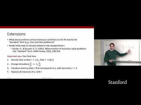
Time rescaling is used to transform problems with free final time into a standard form where tau = t / tf, making the final time 1.
A dummy state variable 'r' with trivial dynamics (r_dot = 0) is introduced to represent the final time.

8:52 Example: Particle on a Line with Free Final Time

Revisiting a previous example: controlling a particle from x=10 to x=0 with zero velocity.
The cost functional includes a term for final time and control effort.
This problem has a free final time, requiring the time rescaling and dummy variable trick.

10:40 Deriving Optimality Conditions for Particle Control

System dynamics: x1_dot = x2, x2_dot = u.
Hamiltonian: H = 0.5 * u^2 + p1 * x2 + p2 * u.
Optimality conditions: p1_dot = 0, p2_dot = -p1, u = -p2 / b.

17:10 Boundary Conditions for the Particle Problem

Initial conditions: x1(0)=10, x2(0)=0.
Final conditions: x1(tf)=0, x2(tf)=0.
Master boundary condition for free final time: H(tf) + terminal_cost_derivative = 0, leading to -p2^2 * tf / (2b) + alpha * tf = 0.

20:40 Implementing Indirect Methods with SolveBVP

Defining differential equations including the rescaled time dynamics and the dummy variable 'r'.
Boundary conditions are fed to the solver as residuals.
Discretized time array from 0 to 1 is used due to time rescaling.

23:46 Numerical Solution and Verification

Running the solver yields a final time tf = 4.47.
This matches the analytical solution (1800 * b/a)^(1/5).
State variables x1 and x2, and control 'u' are visualized.

25:40 Transition to Direct Methods: Strengths and Popularity

Indirect methods require deriving optimality conditions, which can be complex.
Direct methods are increasingly popular due to ease of use and direct discretization.
Indirect methods offer potential for analytical solutions and interpretability (e.g., bang-bang control).

28:21 High-Level Overview of Direct Methods

Direct methods discretize the continuous-time optimal control problem into a nonlinear constrained optimization problem.
Improvements in nonlinear optimization solvers make real-time solutions feasible.
The core idea is to discretize time and solve the resulting optimization problem.

32:35 Two Subcategories of Direct Methods

State and Control Parameterization (Collocation): Both states and controls are optimization variables; dynamics become constraints.
Control Parameterization (Shooting): Only controls are optimization variables; states are computed recursively from dynamics.

35:51 Pros and Cons of Direct Method Families

Control parameterization: Smaller optimization problems (fewer variables), but harder to enforce state constraints.
State and control parameterization: Easier to enforce state constraints by treating states as optimization variables.
Hybrid methods like multiple shooting can combine benefits.

39:14 State and Control Parameterization (Collocation)

Discretizes time using Euler integration and assumes a zero-order hold on controls.
Dynamics are approximated using Euler's method: x(t+dt) = x(t) + dt * f(x, u, t).
The cost integral is approximated as a sum, with integrals over time steps becoming products of cost function and step size 'h'.

48:50 Example: Zermelo's Problem (Crossing the River)

Goal: Cross a river with non-uniform flow, minimizing control effort (angle 'u').
Problem setup: Constant forward velocity 'v', control 'u' is the angle, cost is integral of u^2.
River flow lambda(y) is 0 at banks and maximum in the middle.

55:14 Implementing Zermelo's Problem with State/Control Parameterization

Variables: x, y positions and control 'u' at discrete time steps.
Constraints: Initial (0,0) and final (M,L) positions, control bounds [-umax, umax].
Dynamics constraints: x(i+1) = x(i) + h * (v + lambda(y(i)) * cos(u(i))), y(i+1) = y(i) + h * (lambda(y(i)) * sin(u(i))). (Note: Actual code uses simpler dynamics for illustration).

1:04:01 Challenges with Initial Guess and Constraints

A restrictive umax (0.75) leads to solver failure ('garbage' solution).
Direct methods are sensitive to initial guess quality and problem conditioning.
Solving a relaxed problem (umax=1) first and using its solution as an initial guess for the constrained problem (umax=0.75) enables convergence.

1:13:24 Control Parameterization (Shooting Methods)

Only controls 'ui' are optimization variables; states are computed recursively.
Dynamics are propagated forward from an initial state x0.
This is also known as shooting methods due to the sequential propagation of states.

1:19:10 Implementing Zermelo's Problem with Control Parameterization

Problem definition (dynamics, cost, bounds) is similar to the previous method.
Constraints function depends only on 'u'; dynamics are propagated internally within the constraint evaluation.
This method successfully solves both umax=1 and umax=0.75 cases, potentially less sensitive to initial guess quality.

Summary, takeaways, and chapters were generated by AI from the video's transcript and may contain errors. The video belongs to its creator, Stanford Online.