Stanford AA203 Optimal and Learning-Based Control | Spring 2026 | Lecture 5: Computational Methods

Overview

This lecture from Stanford Online's AA203 course delves into computational methods for optimal control, specifically extending indirect methods to handle bounded controls via Pontryagin's Minimum Principle (PMP). The session details how the stationarity condition on the Hamiltonian is strengthened to a minimization condition, illustrated with minimum time, minimum fuel, and minimum energy problems. It also introduces numerical methods like shooting and collocation for solving the resulting two-point boundary value problems.

Key takeaways

Pontryagin's Minimum Principle strengthens the optimality condition for bounded controls from stationarity to global minimization of the Hamiltonian.
Minimum time problems with bounded controls typically result in 'bang-bang' control strategies, where controls are always at their maximum or minimum limits.
Minimum fuel problems with bounded controls can lead to 'bang-off-bang' strategies, allowing controls to be at their bounds or zero.
Numerical methods like shooting and collocation are essential for solving the complex two-point boundary value problems arising from indirect optimal control methods.
The `scipy.optimize.solve_bvp` function provides a practical tool for implementing these numerical solutions in Python.

Chapters

0:00 Introduction to Open-Loop Control and Indirect Methods

Recap of open-loop control and the distinction between indirect (optimize then discretize) and direct (discretize then optimize) methods.
Introduction to optimality conditions for unbounded controls, defining the Hamiltonian as an analog to the Lagrangian.
The Hamiltonian is defined as state cost + costates * dynamics, with costates analogous to Lagrange multipliers.

3:37 Extending Optimality Conditions for Bounded Controls

Focus shifts to optimal control problems with bounded controls, a common practical constraint.
State constraints are mentioned but not covered due to complexity and indirect methods not being the primary tool for them.
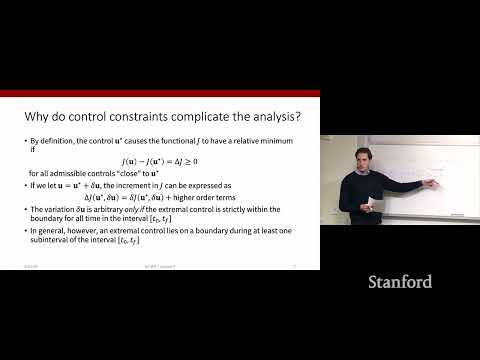
The core idea is that bounds on controls complicate the analysis by restricting admissible variations.

18:22 Finite Dimensional Optimization with Boundaries

Recap of finite dimensional optimization: gradient of f = 0 for unconstrained problems.
With boundaries, the increment of the function must be >= 0 for admissible displacements.
Boundary points can be local minima even if the gradient is not zero.

25:50 Calculus of Variations and Bounded Controls

The same intuition applies to infinite-dimensional optimization (calculus of variations).
The variation of the cost functional (delta j) must be >= 0 for admissible variations.
When controls are at a boundary, admissible variations are one-sided, breaking the assumption of arbitrary variations.

35:22 Pontryagin's Minimum Principle (PMP)

The condition delta j >= 0 leads to strengthening the stationarity condition on the Hamiltonian.
The optimal control u must be a global minimizer of the Hamiltonian, not just a stationary point.
This strengthens the third algebraic condition derived from the optimality conditions.

38:56 Example: Minimum Energy Problem with Bounded Controls

System: second-order linear dynamics, cost functional is quadratic in controls (minimum energy).
Constraint: |u| <= 1.
The Hamiltonian is defined, and the third condition requires minimizing H with respect to u.

54:04 Minimizing the Hamiltonian for Minimum Energy

The minimization problem boils down to minimizing 1/2 u^2 + p2*u.
Setting the derivative to zero gives u_star = -p2.
Case analysis is performed based on the bounds [-1, 1] and the value of -p2.

57:27 Control Profile for Minimum Energy Problem

If -p2 is within [-1, 1], u_star = -p2.
If -p2 < -1, u_star = -1.
If -p2 > 1, u_star = 1.
This results in a linear control profile that saturates at the bounds.

1:08:28 Summary of Minimum Energy Control Profile

The derived control profile is linear between -1 and 1, saturating at the bounds.
Pontryagin's additional conditions are mentioned (e.g., constant Hamiltonian if final time is fixed and H is time-invariant).
These additional conditions help further characterize the solution.

1:10:47 Archetype Problem: Minimum Time

Objective: Reach the origin from an arbitrary state x0 as fast as possible.
Cost functional: Integrate 1 over time (minimize tf).
System: Control affine (linear in u, potentially nonlinear in x).
Control bounds: Mi- <= ui <= Mi+.

1:15:51 Hamiltonian for Minimum Time Problem

Hamiltonian = 1 (state cost) + p^T * (A*x + B*u).
The term p^T * B*u depends on u.
Minimizing the Hamiltonian requires minimizing p^T * B*u with respect to u.

Summary, takeaways, and chapters were generated by AI from the video's transcript and may contain errors. The video belongs to its creator, Stanford Online.