Stanford AA203 Optimal and Learning-Based Control | Spring 2026 | Lecture 4: Indirect Methods

Overview

This lecture from Stanford's AA203 Optimal and Learning-Based Control course, taught by Stanford Online, delves into indirect methods for optimal control, building upon the fundamental theorem of calculus of variations. It explains how to derive necessary optimality conditions, exemplified by finding the shortest path between two points, and then extends these methods to handle free boundary conditions and system dynamics constraints using Lagrangians and costate variables. The lecture concludes by outlining the derivation of optimality conditions for optimal control problems with unbounded controls, introducing the Hamiltonian and its application to a particle dynamics example.

Key takeaways

Indirect methods for optimal control transform infinite-dimensional optimization problems into solving differential equations derived from necessary optimality conditions.
The Euler equation, derived from the calculus of variations, is a key tool for finding optimal paths, exemplified by the shortest path problem yielding a straight line.
Generalized boundary conditions are crucial for determining integration constants when final states or times are not fixed, derived from variations in the Hamiltonian.
The Hamiltonian formulation (H = g + p^T*f) provides a systematic way to derive optimality conditions (x_dot, p_dot, dH/du=0) for optimal control problems.
The example of a particle controlled by acceleration demonstrates how to apply the Hamiltonian method, solve the resulting differential equations, and use boundary conditions to find the optimal control and trajectory.

Chapters

0:00 Roadmap and Introduction to Indirect Methods

Recap of the roadmap, focusing on open-loop optimal control methods.
Indirect methods define necessary optimality conditions for infinite-dimensional optimization problems.
Key concept: extending finite-dimensional optimization to functionals (functions of functions).

2:26 Fundamental Theorem of Calculus of Variations

The variation of the cost functional J must vanish at an optimal solution x*.
This condition is analogous to the gradient being zero in finite-dimensional optimization.
This theorem provides necessary but not always sufficient conditions for optimality.

5:18 Simplified Optimal Control Problem and Euler Equation

Focus on a simplified problem where the state trajectory is directly controlled.
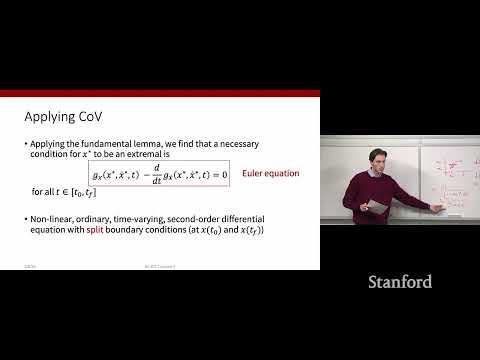
Derivation of the Euler equation as an actionable optimality condition.
The Euler equation is a second-order nonlinear ODE with split boundary conditions.

10:31 Example: Shortest Path Between Two Points

Defining the functional J as the integral of ds, representing path length.
Approximating ds using Pythagorean theorem: ds = sqrt(dt^2 + dx^2).
Functional J = integral(sqrt(1 + x_dot^2)) dt.

17:03 Applying the Euler Equation to Shortest Path

Calculating partial derivatives of g(x, x_dot) = sqrt(1 + x_dot^2).
g_x = 0, g_x_dot = x_dot / sqrt(1 + x_dot^2).
The Euler equation simplifies to d/dt(g_x_dot) = 0.

23:26 Solving the Euler Equation for Shortest Path

The derived Euler equation is x_double_dot = 0.
Integrating twice yields x(t) = c1*t + c2, the equation of a line.
This proves that a straight line is a candidate for the shortest path.

28:22 Extending to Optimal Control Problems

Transitioning from calculus of variations to actual optimal control problems.
Relaxing assumptions on fixed boundary conditions (final time and state).
Need for more sophisticated boundary conditions to determine constants of integration.

33:41 Generalized Boundary Conditions

A general boundary condition equation involving variations in xf and tf.
Specific cases arise depending on whether xf and tf are fixed or free.
Example: If tf is fixed and xf is free, then dg/dx_dot(tf) = 0.

39:01 Example: Shortest Path to a Free Final State

Problem: Find shortest path from x(0)=1 to a free x(tf) at fixed tf=5.
Euler equation still yields x(t) = c1*t + c2.
Initial condition x(0)=1 implies c2=1, so x(t) = c1*t + 1.

45:31 Applying Generalized Boundary Conditions

Case: tf fixed, xf free. Additional condition: dg/dx_dot(tf) = 0.
dg/dx_dot = x_dot / sqrt(1 + x_dot^2).
Setting dg/dx_dot(tf) = 0 implies x_dot(tf) = 0.

48:42 Solving for Constants with Free Final State

x(t) = c1*t + 1, so x_dot(t) = c1.
x_dot(tf) = 0 implies c1 = 0.
Solution: x(t) = 1, a constant path.

52:17 Extension: Constraints on Dynamics

Considering constraints that link the function (states) with its derivative (controls).
Introducing w = (x, u) and an augmented integrand g(a) = g + p^T * f.
This is analogous to using Lagrange multipliers in finite-dimensional optimization.

57:20 Hamiltonian Formulation for Optimal Control

Defining the Hamiltonian H = g(x, u, t) + p^T * f(x, u, t).
Optimality conditions involve Euler-Lagrange equations on the Hamiltonian.
Conditions: x_dot = dH/dp, p_dot = -dH/dx, dH/du = 0.

1:03:43 Optimal Control Problem with Unbounded Controls

Objective: Minimize J = integral(g(x, u, t)) dt + terminal_cost(x(tf), tf).
System dynamics: x_dot = f(x, u, t).
Focus on deriving necessary optimality conditions without control bounds.

1:06:58 Optimality Conditions for Unbounded Controls

Define Hamiltonian H = g(x, u, t) + p^T * f(x, u, t).
Conditions: x_dot = dH/dp, p_dot = -dH/dx, dH/du = 0.
Boundary conditions depend on whether x(tf) and tf are fixed or free.

Summary, takeaways, and chapters were generated by AI from the video's transcript and may contain errors. The video belongs to its creator, Stanford Online.