Stanford AA203 Optimal and Learning-Based Control | Spring 2026 | Lecture 13: Intro to Learning

Overview

This lecture introduces learning-based control, shifting from optimal control methods that assume known dynamics to scenarios where system dynamics are unknown. It categorizes approaches to uncertainty into feedback control, robust control, and data-driven methods. The focus then narrows to data-driven techniques, specifically system identification using linear regression and adaptive control, exemplified by Model Reference Adaptive Control (MRAC). The lecture details the mathematical framework for linear regression-based system identification and then delves into MRAC's stability analysis using Lyapunov functions, demonstrating how to adapt controller parameters online to unknown system dynamics.

Key takeaways

Learning-based control addresses systems with unknown dynamics, moving beyond traditional optimal control methods.
System identification, using techniques like linear regression, estimates system dynamics from collected data.
Model Reference Adaptive Control (MRAC) achieves stability by online adaptation of controller parameters to unknown system dynamics, proven via Lyapunov stability.
The MRAC stability analysis for a double integrator with unknown mass uses a candidate Lyapunov function V = ½ms² + (1/2γ)m̃², showing convergence of the tracking error (x̃) to zero.
Lyapunov stability analysis is crucial for proving the stability of coupled systems involving the plant, controller, and adaptation mechanism in adaptive control.

Chapters

0:00 Transition to Learning-Based Control

Previous lectures covered optimal control (open-loop and closed-loop methods) and Model Predictive Control (MPC).
These methods assumed known system dynamics.
The second part of the course relaxes this assumption, focusing on learning-based control where dynamics are unknown.

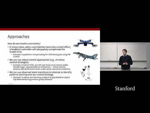
3:26 Approaches to System Uncertainty

Simple feedback control can compensate for small unmodeled effects (e.g., PID control).
Robust control (e.g., min-max formulation) handles uncertainty by considering worst-case scenarios, potentially leading to conservative behavior.
Data-driven methods leverage collected state transitions to learn approximate models of dynamics.

12:23 Two Families of Learning-Based Control

Directly improve the controller using measurements or collected data.
Learn an approximate model of dynamics from data and then use this model to improve the controller (intermediate step: system identification).

14:05 Today's Focus: Adaptive Control and System Identification

Direct adaptive control and indirect adaptive control.
System identification.
Future topics: imitation learning, model-free and model-based reinforcement learning.

15:22 Modalities of Learning Experience

Zero-episode case (offline): Learn from a pre-collected dataset.
One-episode case (online): Adapt and learn in real-time while controlling the system.
Multiple-episode case: Learn across repeated interactions with an environment (classical RL).

26:53 System Identification: Learning Dynamics from Data

Goal: Build a data-driven model of dynamics using past experiments or behaviors.
Use the learned model as a proxy for control design.
Problem: Missing dynamical model, learn approximation from prior data.

28:35 Linear Regression for System Identification

Model: y = θᵀz + ε, where y is output, z is input, θ are parameters, ε is noise.
Data set D = {(zᵢ, yᵢ)} for i=1 to N.
Objective: Minimize least squares loss: ||y - Zθ||².

33:22 Least Squares Solution for Linear Regression

Convex optimization problem.
Solution derived by setting gradient with respect to θ to zero.
Estimator: θ̂ = (ZᵀZ)⁻¹Zᵀy.

37:06 Applying Linear Regression to System Dynamics

Model: x(t+1) = Ax(t) + Bu(t) + ε(t).
Data collection: Trajectories of states x(t) and controls u(t) to predict next state x(t+1).
Repurposed as a regression problem: map (x(t), u(t)) to x(t+1).

42:17 Comments on System Identification Estimator

Recursive formulations exist to avoid expensive matrix inversion for large datasets.
Discrete-time and continuous-time equivalents.
The estimator is the Best Linear Unbiased Estimator (BLUE) under common noise assumptions.
If noise is Gaussian, it's also the Maximum Likelihood Estimator (MLE).

45:23 Convergence Properties of the Estimator

Mean of θ̂ converges to true θ if noise is zero-mean.
Covariance of θ̂: σ² * (Σ(zᵢzᵢᵀ))⁻¹.
Covariance goes to zero as N increases, provided persistent excitation (non-trivial system probing).

1:00:09 Practical Questions in System Identification

Data budget: How much data is needed?
Quantifying 'good' parameter estimation vs. control performance.
Model family expressivity: Does the chosen model class (e.g., linear) match reality?

1:07:08 Introduction to Adaptive Control

Falls into the one-episode (online adaptation) setting.
Improves control in real-time as the system operates.
Can directly improve controller or learn a model first.

1:08:30 Model Reference Adaptive Control (MRAC)

Four key elements: plant with unknown parameters, reference model (desired output), feedback control law with adjustable parameters, adaptation mechanism.
Focuses on proving stability of the coupled system (plant, controller, adaptation mechanism).

1:10:45 Lyapunov Stability Recap

Tool for analyzing stability of autonomous systems.
Requires finding a Lyapunov function V(x) that is positive definite, has a negative definite derivative V̇(x), and is radially unbounded.

1:18:25 Lyapunov Stability Example: Mass-Spring-Damper

System: mẍ = -dẋ - kx + f.
Candidate Lyapunov function: Energy E = ½kx² + ½mẋ².
Derivative V̇ = -dẋ² (negative definite if d>0), confirming stability to the zero equilibrium point.

Summary, takeaways, and chapters were generated by AI from the video's transcript and may contain errors. The video belongs to its creator, Stanford Online.