Stanford AA203 Optimal and Learning-Based Control | Spring 2026 | Lecture 12: Feasibility of MPC

Overview

This lecture on MPC feasibility and stability by Stanford Online focuses on ensuring that Model Predictive Control systems have feasible solutions at each step and converge to a desired equilibrium. It introduces the concept of control invariance for terminal sets to guarantee persistent feasibility and leverages Lyapunov stability theory to prove convergence. The lecture also touches upon offline computation of MPC and its application to trajectory tracking, highlighting practical considerations for tuning MPC parameters like the terminal set (Xf) and terminal cost (P).

Key takeaways

Persistent feasibility in MPC is guaranteed if the terminal set Xf is control invariant.
The optimal cost function J* of an MPC problem can serve as a Lyapunov function to prove stability.
For stable linear systems, choosing Xf as the maximal positive invariant set and P from the Lyapunov equation ensures stability.
For unstable linear systems, using LQR closed-loop dynamics for Xf and the Riccati equation for P ensures stability.
Explicit MPC converts the online optimization problem into a lookup table, useful for safety-critical applications despite potential complexity.
Trajectory tracking with MPC is best formulated using delta controls to avoid oscillations between tracking error and control effort penalties.

Chapters

0:00 Introduction to MPC Feasibility and Stability

Review of persistent feasibility as a key property for MPC.
Introduction to stability: ensuring MPC actions are useful and lead to convergence.
Overview of topics: offline computation, trajectory tracking, and practical relevance.

2:18 Feasibility Lemma: Control Invariance and Persistent Feasibility

Recap of concepts: one-step controllable set, controlling variance set, positive invariant set, feasibility set.
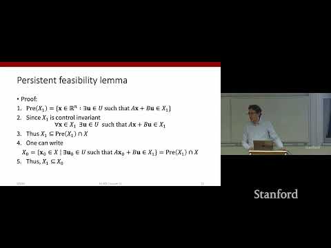
Statement of the lemma: if X1 (truncated feasibility set) is control invariant, MPC is persistently feasible.
Proof involves relating X1 to the one-step controllable set of X1 and X0.

19:11 Theorem: Terminal Set Control Invariance Guarantees Feasibility

Theorem: If the terminal set Xf is control invariant, then the MPC law is persistently feasible.
The origin (0) is a trivial control invariant set.
Discussion on choosing Xf: origin guarantees feasibility but can be suboptimal; relaxed Xf is preferred.

26:49 Proof of Terminal Set Control Invariance Theorem

Proof strategy: show Xf control invariant implies XN-1 control invariant, recursively down to X1.
XN-1 is defined as a truncated feasibility set for a one-step horizon.
If Xf is control invariant, then XN-1 is also control invariant, leading to X1 being control invariant.

37:09 Introduction to Lyapunov Stability Theory

Transition to the topic of stability for MPC.
Intuition of Lyapunov stability: if starting near an equilibrium, will you return without wild trajectories?
Lyapunov's idea: use an energy-like function that decreases along system trajectories to infer stability.

45:01 Lyapunov Stability Theorem Statement

For a system XK+1 = F(XK) with equilibrium at 0.
A function V(X) is a Lyapunov function if V(0)=0, V(X)>0 for X!=0, and V decreases along trajectories.
If such a V exists, the equilibrium is asymptotically stable.

50:32 Celebrated Stability Theorem for MPC

Assumptions: LQR setting (quadratic cost), positive definite R, Q, P, origin in X, Xf, U, and a specific Lyapunov-like condition (Assumption 4).
Theorem: If assumptions hold, the origin is asymptotically stable with domain of attraction X0.
The optimal cost J* is proposed as a Lyapunov function.

1:00:26 Proof of MPC Stability Theorem: J* as Lyapunov Function

Show J*(X) is 0 at origin and positive elsewhere.
Prove J*(X1) < J*(X0) along closed-loop trajectories using Assumption 4 and control invariance of Xf.
The inequality J*(X1) <= J*(X0) - C(X0, U0) + (terms <= 0) implies strict decrease.

Summary, takeaways, and chapters were generated by AI from the video's transcript and may contain errors. The video belongs to its creator, Stanford Online.