Stanford AA203 Optimal and Learning-Based Control | Spring 2026 | Lecture 11: Introduction to MPC
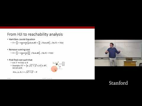 Watch on YouTube →
Overview
This lecture introduces Model Predictive Control (MPC) as a framework that combines the speed of open-loop control with the power of closed-loop methodologies. It contrasts MPC with Hamilton-Jacobi-Isaacs (HJI) reachability analysis, which computes reachable sets (avoidance and reach sets) using differential games and the HJI equation. The lecture details how to formulate reachability problems by removing running costs and defining final costs based on set membership, illustrating with a unicycle example and a two-airplane collision avoidance scenario. MPC is then presented as a receding horizon optimization strategy that repeatedly solves finite-horizon optimal control problems, applying only the first control action and replanning based on new state measurements, making it intuitive and widely applicable, especially for systems with constraints.
Key takeaways
- Hamilton-Jacobi-Isaacs (HJI) equation, through the level set method, can compute backward reachable sets by encoding set membership as a cost function.
- Reachable tubes extend reachable sets to ensure safety across an entire trajectory, not just the endpoint, by modifying the cost function to minimize the minimum `h(x(t))`.
- Model Predictive Control (MPC) is a framework that repeatedly solves finite-horizon optimal control problems, applying only the first control action and replanning based on new state measurements.
- MPC's core idea is receding horizon optimization, balancing computational cost with performance by solving open-loop problems that effectively create a closed-loop system.
- Control invariant sets are crucial for guaranteeing persistent feasibility in MPC; if the set of states from which an N-1 horizon problem is feasible is control invariant, the MPC law is guaranteed to be feasible.
- Tuning MPC involves balancing lookahead capabilities (horizon length, terminal cost/constraint) against computational cost to ensure both persistent feasibility and stability.
Chapters
- Reachability theory uses the Hamilton-Jacobi-Isaacs (HJI) equation to compute reachable sets.
- Avoidance sets: states from which there exists a disturbance to reach the target set.
- Reach sets: states from which for all disturbances, a control can reach the target set.
- Avoidance set: states from which any control input, under any disturbance, leads to the target set at t=0.
- Reach set: states from which for all disturbances, there exists a control input to reach the target set at t=0.
- Avoidance sets constrain initial conditions to be outside; reach sets require initial conditions to be inside.
- HJI equation can compute backward reachable sets procedurally.
- Involves solving a differential game with two players: controller (us) and nature (disturbance).
- Boolean outcome of set membership is encoded by removing running cost and using final cost for set definition.
- Boolean set membership can be represented by a cost function `h(x)`.
- Target set T is the zero level set of `h(x)`, where `x` is in T iff `h(x) <= 0`.
- Example: A circle of radius R is defined by `h(x, y) = x^2 + y^2 - R^2`.
- Set membership is defined by `h(x) <= 0`.
- For avoidance, player 1 maximizes `h` (stay outside), player 2 minimizes `h` (force inside).
- The magnitude of `h` provides a safety buffer or 'how unsafe' the state is.
- Avoidance set computation: minimax problem to maximize `h`.
- Reach set computation: min-max problem to minimize `h` (swapping player roles).
- HJI equation is used with zero running cost and `h(x)` as the boundary condition.
- Static reachability defines initial states for desirable final conditions.
- Reachable tubes consider safety across the entire trajectory, not just the endpoint.
- Objective becomes minimizing the minimum value of `h(x(t))` over the horizon.
- Caring about the entire trajectory requires a modified cost function: `min_tau h(x(tau))`.
- This strengthens the safety objective by ensuring `h(x(t)) > 0` for all `t`.
- The HJI equation becomes more complex due to this additional minimization.
- BRS: set of initial states ensuring safety at the end of the horizon.
- BRT: set of initial states ensuring safety throughout the entire horizon.
- Both BRS and BRT computation yield the set and the optimal control policy.
- Two airplanes with unicycle dynamics, controlled heading `theta`.
- Collision defined as relative distance < r.
- Goal: compute the set of initial conditions for aircraft B to avoid collision with A.
- The computed backward reachable set has a complex, non-circular shape in relative state-space (x, y, z).
- The shape depends on relative heading `z` and longitudinal/lateral separation.
- A 'protrusion' indicates increased separation needed when aircraft are on a collision course.
- The shape of the backward reachable set evolves with the time horizon.
- For stationary problems, the set often converges to a constant after a transient period.
- This indicates that beyond a certain time, additional planning time offers no further safety benefit.
- Simulations show trajectories starting inside or outside the BRS.
- Starting outside guarantees avoidance; starting inside may lead to persistent collision risk.
- A trajectory briefly entering the protected space highlights the need for BRT for stricter safety.
- Solving HJI PDEs is computationally hard, limited by the curse of dimensionality (typically 5-6D state space).
- Approximation techniques (neural networks, sampling-based methods) are used for higher dimensions.
- Python package 'HJ reachability' provides an exact solver for lower dimensions.
- MPC aims to combine open-loop speed with closed-loop power.
- It's a framework, not a single strategy, widely used since the '70s/'80s.
- Originally developed for chemical engineering due to constraint handling needs and slower dynamics.
- MPC solves an open-loop optimal control problem over a finite horizon `Np` at each time step `t`.
- Only the first control action `u(t)` is applied.
- The system state is measured at `t+1`, and the entire problem is recomputed from scratch.
Summary, takeaways, and chapters were generated by AI from the video's transcript and may contain errors. The video belongs to its creator, Stanford Online.