Stanford AA203 Optimal and Learning-Based Control | Spring 2026 | Lecture 1: Course Overview

Overview

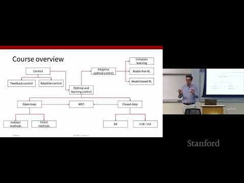
Marco Pavone introduces AA203 Optimal and Learning-Based Control, a course covering both classical optimal control (open-loop, closed-loop, MPC) and data-driven approaches (imitation learning, reinforcement learning). The course emphasizes a unified framework, blending theoretical and practical aspects with Python coding. Grading includes four problem sets (80%) and a final exam (20%), with up to 5% bonus for participation. Prerequisites include calculus and linear algebra, with familiarity in optimization and machine learning being beneficial.

Key takeaways

AA203 covers both traditional optimal control (open-loop, closed-loop, MPC) and modern data-driven methods (imitation, reinforcement learning).
The course emphasizes a unified framework, blending theory and Python implementation, with problem sets and a final exam.
Prerequisites include strong calculus and linear algebra; familiarity with optimization and ML is beneficial.
Optimal control problems are formulated with system models (ODEs), constraints, and performance criteria (terminal/stage-wise costs).
Open-loop control is time-dependent, while closed-loop control is state-dependent (policy), with MPC offering a hybrid approach.
The course will build from classical optimization techniques (unconstrained/constrained) to tackle infinite-dimensional optimal control problems.

Chapters

0:00 Introduction to Marco Pavone and Course Mechanics

Marco Pavone, professor in Aeronautics and Astronautics, leads AA203.
Coursework includes four problem sets (Python coding & theory) and a final exam.
Grading: 80% problem sets (20% each), 20% final exam, up to 5% bonus for participation.
Six free late days available, max two per assignment.

3:15 Course Materials and Recitations

All necessary materials provided on the website, including lecture slides and course notes.
Optional books and references are available for deeper study.
Recitations held for the first four weeks on Fridays (1:30-2:30 PM) to cover foundational tools like Jags and regression models.

5:17 Prerequisites for Success in AA203

Strong comfort with multivariable calculus and ordinary differential equations is required.
Solid understanding of linear algebra is essential.
Familiarity with optimization, machine learning, and control theory is beneficial but not mandatory.

7:01 Homework 0: Self-Assessment Tool

Homework 0 is ungraded and serves as a self-assessment for readiness.
Solutions will be provided; it's available on the website.
Encouraged to solve without AI tools like ChatGPT to identify knowledge gaps.

8:35 Course Philosophy: Breadth Over Depth

The course aims for a broad overview of optimal and learning-based control techniques.
Covers 50 years of optimal control literature and current AI/robotics topics.
Acknowledges a trade-off between breadth and depth, requiring self-study for deeper dives.

10:12 Course Challenge and Structure Overview

The course is considered challenging due to the variety of topics covered.
Requires knowledge in calculus, statistical analysis, and other dimensions.
Mechanics of the course include problem sets and a final exam.

12:04 Motivation: The Essence of Control Systems

Control involves acting on a system (physical or abstract) to achieve a desired response.
Standard setup: system, sensors, reference (goal), controller, control action, output.
Human closed-loop control example: eyes as sensors, planning movement to a door.

16:41 Control System Examples and Modeling Pragmatism

PID controllers are a common example in frequency domain control.
Room temperature control: home as system, thermostat as reference.
Control modeling is pragmatic; models can be simplified or learned from data, unlike detailed thermodynamic models.

19:00 Challenges in Control Systems

Challenges include disturbances (e.g., wind gusts) and sensor noise.
Classical control addresses stability, tracking, disturbance rejection, and robustness.
Robustness ensures performance despite model inaccuracies or system changes over time.

23:22 Limitations of Classical Control and Course Objectives

Classical control often overlooks performance optimization (e.g., minimizing control effort).
Planning the reference signal (e.g., aircraft trajectory) is not typically covered.
The course addresses how to optimize performance, learn models from data, and incorporate planning.

25:17 Optimal and Learning-Based Control: Core Concepts

Optimality focuses on the best way to control a system, often defined by a performance objective.
Learning addresses adapting controllers based on acquired data when models are unknown or change.
The field dates back to the Cold War, with pioneers Richard Bellman and Pontryagin.

28:24 Open-Loop vs. Closed-Loop Optimal Control

Open-loop control computes a sequence of actions assuming no further information is gathered (e.g., planning a path with eyes closed).
Closed-loop control involves continuous measurement and re-optimization of actions.
Open-loop is computationally efficient but less robust; closed-loop is powerful but more complex.

33:32 Model Predictive Control (MPC) and Data-Driven Control

MPC bridges open-loop and closed-loop control by re-solving open-loop problems iteratively.
The second half of the course focuses on data-driven control where models are inferred from data.
Methods include imitation learning (mimicking expert behavior) and reinforcement learning (trial-and-error).

35:06 Data-Driven Control Methodologies

Imitation learning mimics optimal policies from demonstrations.
Reinforcement learning involves learning through trial and error (model-based and model-free).
Hybridization of techniques (e.g., imitation learning to bootstrap RL) is common.

40:26 Course Goals: Theory, Implementation, and Unified Framework

Goal: Learn theoretical and implementation aspects of optimal and learning-based control.
Provide a unified framework connecting classical optimal control, DP, and RL.
Empower designers to choose the best tool for a given problem.

42:21 Defining Optimality: Performance Metrics

Optimality is defined by a performance index chosen by the designer.
Metrics can include stability, control effort, time to completion, and tracking error.
Trade-offs between conflicting objectives (e.g., speed vs. energy) are managed through the performance index.

44:18 The Optimal Control Problem Formulation

Three main ingredients: system model, constraints, and performance criteria.
System model: typically a set of ordinary differential equations (ODEs) describing state evolution.
Constraints: initial conditions, final conditions, state bounds, control bounds.

46:52 Mathematical Model: Ordinary Differential Equations (ODEs)

ODEs (x_dot = f(x, u, t)) describe how system state 'x' evolves based on control 'u' and time 't'.
An ODE provides a mechanism to predict the future state of the system.
The course assumes 'f' can be non-linear, moving beyond standard linear control assumptions.

53:57 Notation for State and Control Variables

Bold vectors 'x' and 'u' represent sets of state and control variables, respectively.
The system dynamics 'f' can be a concatenation of functions for multiple state variables.
The model can explicitly depend on time 't', indicating time-varying system behavior.

57:06 Example: The Double Integrator System

A cart on a plane controlled by force (acceleration).
Second-order ODE (s_double_dot = input) can be converted to two first-order ODEs by adding velocity 'v' as a state.
Augmented state vector: [displacement, velocity].

1:02:16 Linear Systems Representation

Linear systems can be represented in matrix form: x_dot = Ax + Bu.
A is the state matrix, B is the input matrix.
This standard form is used in classical control theory.

1:03:43 Constraints in Optimal Control

Constraints include initial/final conditions, state bounds (avoiding bad regions), and control bounds.
Examples: not hitting a wall, actuator limits, landing on a specific point.
Admissible control/trajectory satisfies all constraints at all times.

1:07:17 Performance Measure: Terminal and Stage-wise Costs

Performance measure quantifies 'best' control; typically minimized.
Terminal cost (h(x_tf, tf)) penalizes the final state at the final time.
Stage-wise cost (integral of g(x, u) dt) accumulates costs incurred over time (e.g., control effort, tracking error).

Summary, takeaways, and chapters were generated by AI from the video's transcript and may contain errors. The video belongs to its creator, Stanford Online.