RAS455 9 16

Overview

The class derives forward and inverse kinematics for a three-joint R-perpendicular-R-parallel-R robot, using coordinate-frame rules, homogeneous transformations, and MATLAB symbolic computation. It also applies the workflow to a two-revolute-joint robot, demonstrates how link lengths and joint angles determine end-effector position, and assigns a prior R-perpendicular-P robot as a MATLAB quiz problem.

Key takeaways

For the R-perpendicular-R-parallel-R example, forward kinematics give Px = cos(θ1)[a2 cos(θ2) + a3 cos(θ2 + θ3)], Py = sin(θ1)[a2 cos(θ2) + a3 cos(θ2 + θ3)], and Pz = a1 + a2 sin(θ2) + a3 sin(θ2 + θ3).
Coordinate-frame placement determines each homogeneous transform: joint axes define Z, each subsequent X intersects and is perpendicular to the preceding Z, and aligned neighboring frames use an identity projection matrix.
A homogeneous transformation's upper-left 3×3 block describes orientation, while the first three entries of its final column give position in the reference frame.
MATLAB's syms, simplify, subs, and vpa functions support symbolic forward-kinematics derivation and numeric evaluation without hand-expanding long matrix products.
Forward kinematics gives a position for specified joint angles, whereas inverse kinematics can yield multiple candidates or no solution; candidates must be checked against physical reachability, collisions, and joint limits.
For a1 = 135 mm, a2 = 165 mm, a3 = 170 mm and angles (0°, 35°, −60°), the demonstrated end-effector position is approximately (289.23, 0, 157.7) mm.

Chapters

0:00 Class Goal: Solve a Three-Revolute-Joint Robot

The class focuses on forward and inverse kinematics for a robot with three revolute joints.
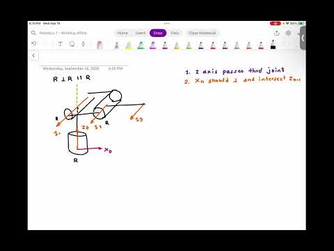
The example is labeled R-perpendicular-R-parallel-R: joint 1 is perpendicular to joint 2, while joints 2 and 3 are parallel.

3:00 Reduce the Physical Robot to a Kinematic Diagram

A kinematic diagram represents a robot as joints connected by links, simplifying its physical construction.
The end effector is attached at the last frame and may hold a gripper, pen holder, or soft gripper.

6:00 Place Z-Axes Along the Revolute Joint Axes

The first coordinate-frame rule places each Z-axis along its corresponding joint axis.
The example labels the joint axes Z0, Z1, and Z2, with Z3 assigned to the end-effector frame despite there being no fourth joint.

10:00 Choose X-Axes Perpendicular to Adjacent Z-Axes

For each frame after the base, Xn must intersect and be perpendicular to Z(n−1).
Because no preceding joint axis exists for frame 0, X0 can be chosen conveniently; the class selects one direction for the diagram.

12:00 Complete the Right-Hand Coordinate Frames

X1, X2, and X3 are selected to satisfy the perpendicular-and-intersecting rule for the preceding Z-axis.
The right-hand rule determines each remaining Y-axis; the selected frames 1, 2, and 3 are aligned with one another.

15:00 Define Link Offsets and Identify Frame Alignment

The diagram assigns link distances a1, a2, and a3 between successive frame origins.
A rotation matrix must be combined with a projection matrix; aligned frames produce an identity projection matrix, while frames 0 and 1 require a non-identity projection.

16:00 Assign Joint Angles and Set Up the First Rotation

The joint variables are θ1, θ2, and θ3, with positive directions established using the right-hand rule.
Because revolute-joint rotation occurs about Z, each local rotation uses the standard Z-axis sine-and-cosine matrix.

20:00 Derive the Frame-0-to-Frame-1 Transformation

The projection of frame 1 onto frame 0 accounts for their differing axis directions before forming R₀₁.
The homogeneous transformation H₀₁ combines that rotation with translation [0, 0, a1], placing frame 1 a1 units along Z0.

26:00 Derive the Frame-1-to-Frame-2 Transformation

Frames 1 and 2 are aligned, so their projection matrix is the identity and the rotation remains the standard Z-axis rotation by θ2.
The link offset resolves into a2 cos(θ2) along X1 and a2 sin(θ2) along Y1, with zero offset along Z1.

34:00 Derive the Frame-2-to-Frame-3 Transformation

Frames 2 and 3 are also aligned, making their projection matrix an identity matrix.
The final link offset is expressed as a3 cos(θ3) along X2 and a3 sin(θ3) along Y2, with no Z2 displacement.

41:00 Build the End-Effector Transform from Three Links

The end effector is located at the origin of frame 3, so its pose relative to the base is H₀₃.
The forward-kinematics transform is the product H₀₁H₁₂H₂₃; the class begins multiplying these 4×4 matrices by hand.

54:00 Enter the Homogeneous Transforms in MATLAB

The class switches to MATLAB because manually multiplying the three 4×4 transformations becomes cumbersome.
The code defines H₀₁, H₁₂, and H₂₃ using symbolic angles θ1–θ3 and link lengths a1–a3.

1:00:00 Use MATLAB Symbolic Variables and Simplification

MATLAB's syms command keeps a1, a2, a3, t1, t2, and t3 as symbolic variables rather than assigning numeric values.
Multiplying the transforms and applying simplify reduces the symbolic expression to a more readable end-effector pose.

1:05:00 Read Position and Orientation from H₀₃

The upper-left 3×3 block of H₀₃ represents end-effector orientation relative to frame 0.
The last column gives position: its first three entries are the X, Y, and Z coordinates of frame 3's origin.

1:10:00 Interpret the Three-Joint Robot as a Rotating Planar Arm

The parallel axes of joints 2 and 3 make their planar link contributions depend on θ2 and θ2 + θ3.
Joint 1 rotates the planar arm around the base, producing the cosine(θ1) and sine(θ1) factors in the X and Y positions.

1:15:00 Set Up a Numerical Forward-Kinematics Example

The example uses link lengths a1 = 135 mm, a2 = 165 mm, and a3 = 170 mm.
Joint angles are θ1 = 0°, θ2 = 35°, and θ3 = −60°; MATLAB's trigonometric functions require angles in radians.

1:21:00 Check the Numerical End-Effector Position

The position equations are evaluated by substituting the three angles and link lengths into the symbolic expressions.
The expected result is approximately Px = 289.23 mm, Py = 0 mm, and Pz = 157.7 mm.

1:25:00 Frame Inverse Kinematics as Solving for Joint Angles

Inverse kinematics starts with a target position Px, Py, Pz and seeks the corresponding θ1, θ2, and θ3.
The position equations contain sines and cosines of the unknown angles, making them nonlinear transcendental equations rather than a simple linear system.

1:30:00 Use MATLAB solve to Recover Candidate Angles

The MATLAB solve command is applied to the three position equations with θ1, θ2, and θ3 as unknowns.
The demonstration reuses the forward-kinematics target position and converts MATLAB's radian solutions to degrees for comparison.

1:35:00 Filter Multiple Inverse-Kinematics Solutions

For the demonstrated target, MATLAB returns four candidate inverse-kinematics solutions.
A mathematical solution may be mechanically impossible because the robot could collide with itself or exceed its joint limits; an if/else check should select a physically valid configuration.

1:40:00 Revisit the Two-Revolute-Joint R-R Robot

The class returns to an earlier R-parallel-R example with two revolute joints and link dimensions a1, a2, a3, and a4.
Its forward kinematics are obtained by multiplying H₀₁ by H₁₂; the resulting last-column entries provide Px, Py, and Pz.

1:45:00 Implement and Numerically Evaluate the R-R Example

MATLAB is used to verify the two-joint result against the expression previously derived by hand.
A numerical example assigns a1 = 100, a2 = 100, a3 = 135, and a4 = 165, with θ1 = 0° and θ2 = 35°.

1:50:00 Debug MATLAB Substitutions and Transform Entries

The class checks each homogeneous transformation and symbolic substitution when students' outputs fail to match.
The example substitutes both link dimensions and joint angles before calculating Px, Py, and Pz; the expected position is approximately (235, 94, 235) in the stated units.

1:55:00 Attempt Inverse Kinematics for the R-R Robot

After completing the two-joint forward calculation, students are asked to implement inverse kinematics in MATLAB.
The class troubleshoots syntax and debugging errors while students use the forward result as the target for recovering joint angles.

2:04:00 Quiz Assignment: Solve the R-Perpendicular-P Robot

The closing exercise revisits an R-perpendicular-P robot with a revolute angle θ and prismatic displacement d.
Students are asked to use θ = 45°, d = 100 mm, a1 = 100 mm, and a2 = 100 mm to compute Px, Py, and Pz, then recover the joint variables through inverse kinematics.

Summary, takeaways, and chapters were generated by AI from the video's transcript and may contain errors. The video belongs to its creator, ssredkar.