Princeton Intro to Robotics (Fall 2026) | Lecture 8: The Linear Quadratic Regulator (LQR)

Overview

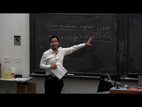
Princeton’s Lecture 8 develops the Linear Quadratic Regulator (LQR) as a principled way to choose a stabilizing feedback controller for a linearized robot model. Given dynamics matrices A and B and designer-selected cost matrices Q and R, LQR solves an algebraic Riccati equation to produce a linear state-feedback law that balances state error against control effort; the lecture also explains practical tuning for a quadrotor and shows applications to aircraft and humanoid robots.

Key takeaways

LQR converts a linearized model x̃̇ = A x̃ + B ũ and quadratic weights Q and R into the feedback law u = u₀ + K*(x − x₀), with K* derived from the algebraic Riccati equation.
Q and R encode engineering priorities: larger Q weights penalize selected state errors more strongly, while larger R weights discourage the corresponding control effort.
For the optimal infinite-horizon controller, the total cost from initial error x̃(0) is x̃(0)ᵀSx̃(0), where S is the stabilizing Riccati solution.
LQR’s global asymptotic stability result applies to the modeled linear system; real quadrotor performance still depends on model accuracy and practical tuning.
In the quadrotor lab, increasing the Z-position weight addresses altitude drift, increasing the Z-velocity weight addresses vertical oscillation, and reducing R allows more aggressive control.
LQR is useful beyond hovering: time-varying LQR can track trajectories, and the lecture’s examples include quadrotors, a prop-hang aircraft, and a humanoid robot.

Chapters

0:00 Feedback Control Recap: Correcting Quadrotor Hover Errors

Feedback control addresses imperfect dynamics and external disturbances, such as wind, by mapping the robot’s measured state to a control input.
A quadrotor hover controller can run a sense–compute–act loop 500 times per second, comparing the current state with the target state.
The preceding lecture’s proportional-derivative controller used position and velocity errors; negative gains turn the vertical-motion model into a stable spring–mass–damper system.

9:10 Why LQR: Choosing Better Gains Than Stability Alone

Many proportional-derivative gain choices can stabilize the same linear system, but they differ in tracking speed and control effort.
LQR selects gains by optimizing a defined performance objective rather than merely requiring stability.
The method assumes a linear model, usually obtained by linearizing nonlinear robot dynamics around a reference state and input.

12:00 Shift the Reference to Zero with Error Coordinates

The lecture defines state error as x̃ = x − x₀ and input deviation as ũ = u − u₀.
For a constant reference, the linearized error dynamics become x̃̇ = A x̃ + B ũ.
A and B encode the linearized system, while x₀ and u₀ represent the desired state and nominal input, such as the thrust needed to hover.

14:10 LQR Cost: Accumulated State Error and Control Effort

The objective integrates penalties over time from zero to infinity, so deviations that persist continue to accumulate cost.
State deviation measures how far the robot is from its target; input deviation penalizes excessive effort relative to the nominal control.
For a hovering quadrotor, the nominal input counters gravity, while the deviation term discourages unnecessarily large thrust or moments.

20:00 Use Q and R to Weight Errors, Units, and Effort

The general quadratic cost uses x̃ᵀQx̃ + ũᵀRũ, with Q weighting state errors and R weighting control-input deviations.
Q and R are designer-selected cost matrices; Q is positive semidefinite and R is positive definite in the standard formulation.
Diagonal weights let designers scale variables with different units, such as quadrotor position in meters, orientation in radians, thrust in newtons, and moments in newton-meters.
Increasing a Q diagonal entry makes its associated state error more costly; increasing an R entry makes the corresponding control action more costly.

27:00 The Cost Function Depends on the Initial State and Applied Inputs

The cost J evaluates a state-and-control trajectory generated from an initial state under a chosen control policy.
LQR seeks a policy that minimizes this accumulated cost for every initial state, rather than tuning a separate input sequence for one starting condition.
Once the initial state, linear dynamics, and control policy are specified, the system dynamics determine the future states needed to evaluate the integral.

39:50 LQR’s Key Result: The Optimal Controller Is Linear

For the infinite-horizon quadratic objective and linear dynamics, the optimal input deviation has the form ũ(t) = K* x̃(t).
At each control cycle, the controller measures the current state error and multiplies it by the same feedback-gain matrix K*.
The resulting law is a proportional state-feedback controller, but its gain is chosen to optimize the specified cost.

42:00 Solve the Algebraic Riccati Equation for S

The first LQR computation solves the continuous-time algebraic Riccati equation: AᵀS + SA − SBR⁻¹BᵀS + Q = 0.
The unknown S is an n × n matrix; A, B, Q, and R come from the linear dynamics and the chosen cost.
Under suitable assumptions, the stabilizing Riccati solution S determines the optimal feedback gains.

45:00 Compute K* and Restore the Reference Input

After solving for S, compute the standard gain K* = −R⁻¹BᵀS.
The full control law adds the nominal input back: u = u₀ + K*(x − x₀), so the correction vanishes at the target state.
For quadrotor hover, u₀ supplies the thrust that balances gravity; K* supplies corrective thrust and moments when the state deviates.

50:00 Fixed-Point LQR Assumptions and Trajectory-Tracking Extensions

The derivation focuses on stabilizing a fixed equilibrium, such as a quadrotor hovering at a specified position and orientation.
Trajectory tracking is also possible: time-varying LQR uses a matrix differential equation and produces a time-varying feedback gain.
In practice, a planner can provide a nominal trajectory and control sequence, while feedback corrects deviations from that plan.

52:20 Numerical Riccati Solvers and Python Sign Conventions

Numerical libraries in Python or MATLAB solve the Riccati equation from A, B, Q, and R, after which the gain follows from matrix multiplication.
The lecture warns that common software uses u = −Kx conventions, while its written convention uses a signed gain differently.
Check the lab’s convention and flip the sign if needed; applying a sign-mismatched gain to the drone can destabilize it.

55:20 Interpret S as the Optimal Cost-to-Go

For an initial state error x̃(0), the minimum infinite-horizon cost is x̃(0)ᵀ S x̃(0).
This quadratic form summarizes the full future penalties on both state deviation and control effort under the optimal controller.
S therefore provides a compact way to compare the expected cost of different initial errors without integrating the entire trajectory.

1:01:20 LQR Stability Guarantee for the Linear System

With the appropriate assumptions and stabilizing Riccati solution, the LQR feedback makes the linear system globally asymptotically stable.
The method combines two results: optimality for the chosen quadratic cost and convergence of the modeled linear system to its equilibrium.
The guarantee applies to the linear model; real robots remain subject to nonlinearities, modeling errors, and unmodeled effects.

1:03:10 Tune Quadrotor Q and R Weights in the Lab

The lab starts from a 12-state quadrotor model and four control inputs, with linearized A and B matrices supplied from the vehicle dynamics.
If altitude drifts, increase the Q weight on Z position; if vertical motion oscillates, increase the weight on Z velocity.
Adjust orientation weights when roll or other angles deviate; R weights regulate control effort, and lowering them permits more aggressive thrust and moments.
Tuning is empirical because the real quadrotor is nonlinear and its model omits effects such as aerodynamics.

1:11:40 LQR Demonstrations: Quadrotors, Prop-Hang Aircraft, and Humanoids

A well-tuned quadrotor LQR tracks periodically changed hover setpoints; reducing R too far can make its control actions jerky.
A fixed-wing aircraft performs a propeller hang using LQR; counter-rotating propellers help cancel yaw torque while specialized wing control surfaces provide rapid attitude control.
A humanoid robot with LQR resists pushes better than a hand-tuned proportional-derivative controller in the demonstrated comparison.
LQR is a strong practical baseline for stabilization, and time-varying LQR can pair with motion planning to track planned trajectories.

Summary, takeaways, and chapters were generated by AI from the video's transcript and may contain errors. The video belongs to its creator, Introduction to Robotics @ Princeton.