Princeton Intro to Robotics (Fall 2026) | Lecture 5: Differential Flatness

Overview

Differential flatness provides a way to plan motions that respect robot dynamics: for a flat system, a sufficiently smooth trajectory in selected outputs determines both the full state and the required controls. For the planar quadrotor, the center-of-mass coordinates x and y are flat outputs, and derivatives through fourth order suffice to reconstruct orientation and thrusts; for a 3D quadrotor, the outputs are x, y, z, and yaw. Planning in flat-output space also lets an RRT generate dynamically executable trajectories, as illustrated by quadrotor trajectory-generation and racing demonstrations.

Key takeaways

For a planar quadrotor, the center-of-mass coordinates x and y are flat outputs: their derivatives determine orientation, the full state, and the two rotor thrusts.
The planar quadrotor needs flat-output derivatives through fourth order because orientation depends on translational acceleration and thrust difference depends on angular acceleration.
A conventional RRT can produce dynamically impossible edges; planning in flat-output space lets a quadrotor execute edges by reconstructing the required state and controls.
For a 3D quadrotor, the flat outputs are x, y, z, and yaw, matching the four control inputs; roll and pitch are recovered from the chosen motion.
Flatness does not remove trajectory smoothness requirements: polynomial segments and derivative-continuity constraints can help make adjacent RRT edges executable.
Differential flatness is powerful but not automatic to establish; finding suitable outputs and reconstruction maps generally requires system-specific analysis.

Chapters

0:00 Why Configuration-Space RRT Edges Can Violate Robot Dynamics

Earlier planning methods included graph search—breadth-first search, depth-first search, and Dijkstra—and RRT growth in continuous configuration space.
A standard RRT extension draws a path from the nearest tree node toward a random sample, but that path may not be physically executable.
A quadrotor cannot translate sideways without tilting, and a conventional car cannot move laterally without omnidirectional wheels.

6:00 Differential Flatness as a Planning Tool for Robots

Differentially flat systems include planar and 3D quadrotors and many car models.
The lecture first develops the idea using a planar quadrotor before giving the general definition.
The central planning opportunity is to choose trajectories in special outputs and derive motions consistent with the robot's dynamics.

7:30 Planar Quadrotor Dynamics from Thrust and Newton's Laws

The planar quadrotor has three configuration variables—x, y, and orientation θ—and two thrust controls, f₁ and f₂.
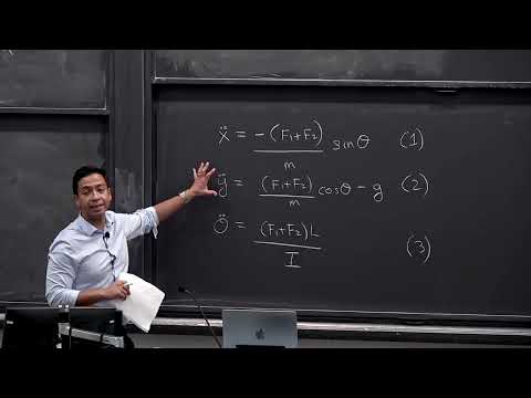
The translational accelerations depend on total thrust f₁ + f₂, mass m, gravity g, and the sine and cosine of θ.
Angular acceleration depends on the thrust difference f₂ − f₁, arm length l, and moment of inertia I.

11:00 The Planar Quadrotor's Flat Output Is Its Center-of-Mass Path

The proposed flat output is z = (x, y), the planar center-of-mass position over time.
Given a trajectory for x(t) and y(t), the goal is to recover both a control trajectory (f₁(t), f₂(t)) and the full state.
The orientation is not independently prescribed; it is determined by the dynamics needed to follow the chosen center-of-mass path.

22:30 Smoothness and Feasibility Conditions for Flat Trajectories

A trajectory cannot demand teleportation or a sharp corner with undefined derivatives; the flat-output path must be sufficiently differentiable.
For the planar quadrotor, reconstructing orientation requires second derivatives of x and y, while computing controls requires derivatives through order four.
A center-of-mass path does not necessarily determine a unique motion or control choice; for example, hovering can allow different orientation behavior.

25:30 Recovering Quadrotor Orientation from Position Acceleration

The translational equations relate ẍ and ÿ to total thrust and orientation θ.
Combining the horizontal and vertical acceleration equations gives θ = atan2(−ẍ, ÿ + g), with mass and total thrust canceling.
Once θ(t) is recovered from x(t) and y(t), differentiating the flat output and θ supplies the six state components: x, y, θ and their velocities.

33:00 Solving for the Two Rotor Thrusts

The known position trajectory supplies the accelerations and, through θ(t), the angular acceleration needed for the dynamics.
The translational equations constrain total thrust f₁ + f₂, while the rotational equation constrains the difference f₂ − f₁.
These two linear equations in f₁ and f₂ can be solved at each time to produce the control-input trajectory.

39:30 General Definition: Flat Outputs, State Map, and Control Map

For dynamics written as ẋ = f(x, u), a flat output z may be a function of state, controls, and—in the general definition—control derivatives.
Flatness requires maps that reconstruct the full state and control from z and a finite sequence of its time derivatives.
In typical robotic examples, including the planar quadrotor, the flat output is simply a selected function or subset of the state.

47:00 Derivative Order and the Limits of Finding Flat Outputs

The reconstruction maps use derivatives up to an order q that depends on the system; for the planar quadrotor, q = 4.
A flat-output trajectory must have the derivatives required by its system's q value.
There is no general algorithm that automatically proves an arbitrary robot is flat; establishing flatness often requires system-specific mathematical insight.

50:00 Flat-Output Dimension Matches the Number of Controls

A stated theorem says the dimension of the flat output equals the dimension of the control input.
For the planar quadrotor, the two outputs x and y correspond to two thrust controls.
This dimension rule helps identify how many independent quantities a candidate flat output must contain.

54:00 3D Quadrotor Flat Outputs: Position and Yaw

The 3D quadrotor has four control inputs, so its flat output has four components: position x, y, z and yaw.
A sufficiently smooth position-and-yaw path determines the required controls and allows roll and pitch to be reconstructed.
The yaw output is independently controllable through differential propeller speeds, while roll and pitch follow from the motion required to accelerate.

59:00 Running RRT in Flat-Output Space

For a 3D quadrotor, RRT can sample and extend trajectories in (x, y, z, yaw) rather than directly in the full configuration space.
Differential flatness provides the controls needed to execute an extension, subject to suitable smoothness at tree vertices.
Time-polynomial trajectory segments can make derivatives easy to compute and enforce continuity constraints, including matching fourth derivatives where required.

1:01:00 Minimum-Snap Quadrotors, Racing, and Flatness-Based Flight Demos

Daniel Mellinger and Vijay Kumar's work, “Minimum Snap Trajectory Generation and Control for Quadrotors,” demonstrated waypoint trajectories and rapid responses to moving objects.
In the demonstrations, planners prescribe x, y, z, and yaw, then use flatness to calculate controls; hoop obstacles can be checked by approximating the drone as a sphere.
The lecture also points to drone racing work by David Scaramuzza's group at the University of Zurich, combining flatness with model predictive control, and shows RRT operating in flat-output space.

Summary, takeaways, and chapters were generated by AI from the video's transcript and may contain errors. The video belongs to its creator, Introduction to Robotics @ Princeton.