Multivariable Calculus Lecture 2 - Oxford Mathematics 1st Year Student Lecture

Overview

Oxford Mathematics develops the workflow for double integrals by first deciding how to integrate over awkward domains and then introducing coordinate changes to simplify both the boundary and the integration measure. Using the disk x^2+y^2 ≤ A^2, the lecture compares Cartesian “vertical slivers” (y = ±√(A^2−x^2), limits x∈[−A,A]) against polar coordinates, deriving the polar area element r d r dθ via a Jacobian and confirming the area is πA^2. It then formalizes the change-of-variables theorem using Jacobians (in 2D and 3D) and applies it to an infinite-domain Gaussian integral, evaluating ∬_{R^2} e^{-(x^2+y^2)} dA to obtain ∫_{-∞}^{∞} e^{-t^2} dt = √π.

Key takeaways

Choosing a coordinate system is a strategy to simplify both the domain boundary and the integration limits: disks become r ≤ A with θ ∈ [0,2π] in polar coordinates.
The correct transformed area element under (x,y) → (r,θ) is dA = r d r dθ, because small polar wedges have approximate area (Δr)(RΔθ), yielding the Jacobian factor r.
For any differentiable invertible change of variables (x,y) → (u,v), area transforms as d x d y = |∂(x,y)/∂(u,v)| d u d v, so Jacobians are the mechanism that fixes scaling after coordinate changes.
The change-of-variables theorem requires a nonzero Jacobian everywhere on the region to ensure the mapping locally stretches space without collapsing it.
Infinite-domain Gaussian integrals can be evaluated by first computing a related 2D integral over R^2 and then taking a square root: ∬_{R^2} e^{-(x^2+y^2)} dA = π implies ∫_{-∞}^{∞} e^{-t^2} dt = √π.

Chapters

0:00 From double integrals over awkward regions to changing coordinates

Recap of choosing integration order for double integrals over domains bounded by functions (sometimes integrate w.r.t. x first, sometimes y).
Motivation to handle more complex domains by changing the coordinate system to simplify boundaries (e.g., disks → polar coordinates).
Plan for a worked example on disk area before moving to a general Jacobian-based framework.

1:15 Disk area in Cartesian coordinates via y = ±√(A^2−x^2)

Problem setup: find area of the disk x^2 + y^2 ≤ A^2, expecting result πA^2.
Writes boundary as y = ±√(A^2−x^2) and integrates using “vertical slithers” with x ∈ [−A, A].
Uses area integral form ∬_D 1 dA = ∫_{x=-A}^{A} (upper−lower) dx = ∫_{-A}^{A} 2√(A^2−x^2) dx.

4:45 Evaluating the Cartesian integral using a trig substitution

Introduces substitution x = A cos θ to rewrite √(A^2−x^2) as A sin θ.
Adjusts limits: x = A corresponds to θ = 0, and x = −A corresponds to θ = π (with θ measured from the x-axis).
Performs the resulting θ-integral and recovers the target area πA^2, validating the method.

6:30 Polar coordinates for the same disk: constant limits and simpler boundaries

Switches to polar coordinates where the boundary becomes r = A (instead of x^2+y^2 = A^2).
Uses θ from 0 to 2π and r from 0 to A, so the region in (r,θ)-space is a rectangle of constant bounds.
Explains that life is easier because limits no longer depend on one variable.

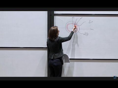
7:05 Deriving the polar area element dA = r d r dθ

Builds polar “area slices” using small changes (Δr, Δθ) that form a wedge and approximates area as (Δr)·(RΔθ).
Concludes that the polar Jacobian contributes the scale factor r to the area element: dA = r d r dθ.
Interprets the integration as summing over radial slithers (fixed r circular rings) as θ varies.

10:00 Formalizing Jacobians: how area elements transform under coordinate maps

Generalizes: under a mapping (x,y) → (u,v), area transforms as dA_uv = |J| d u d v, where J is the determinant of partial derivatives.
Defines the 2D Jacobian J = det(∂(u,v)/∂(x,y)) (or equivalently det(∂(x,y)/∂(u,v)) with a reciprocal relationship).
Motivates the geometric meaning: |J| measures local stretching of small regions.

13:40 Extending Jacobians to 3D and computing the polar Jacobian explicitly

States the 3D analogue: Jacobian is the determinant of ∂(u,v,w)/∂(x,y,z).
For polar mapping x = r cos θ, y = r sin θ, computes the Jacobian determinant to get |J| = r.
Connects directly to the earlier derived area element, confirming consistency: d x d y → r d r d θ.

16:00 Change of variables theorem for integrals with Jacobians

Introduces the change-of-variables theorem for integrals under a differentiable, invertible mapping with nonzero Jacobian.
Gives the equivalence: ∬_S s(u,v) d u d v = ∬_R s(X,Y) |Jacobian| d x d y (with appropriate direction for Jacobians).
Highlights notation: lowercase s on (u,v)-region and uppercase S on (x,y)-region represent the same integrand expressed in different coordinates.

20:40 Gaussian integral on an infinite domain via polar coordinates

Defines infinite integrals as limits: ∫_{-∞}^{∞} f(x) dx = lim_{B→∞} ∫_{-B}^{B} f(x) dx.
Computes I = ∬_{R^2} e^{-(x^2+y^2)} dA using polar variables: integral becomes ∫_{0}^{2π}∫_{0}^{∞} e^{-r^2}·r d r dθ = π.
Uses factorization: (∫_{-∞}^{∞} e^{-t^2} dt)^2 = π, yielding ∫_{-∞}^{∞} e^{-t^2} dt = √π (positivity selects the positive root).

Summary, takeaways, and chapters were generated by AI from the video's transcript and may contain errors. The video belongs to its creator, Oxford Mathematics.