Math 1153 - 6 October 2026 - Section 5.4

Overview

Mike Jacobsen shows how to use a TI-84 calculator’s normal CDF and inverse norm functions to find normal-distribution probabilities and cutoff values more accurately than the 68–95–99.7 empirical rule. Using arsenic concentrations modeled by N(3.2, 1.5) and a 25th-percentile calculation, he demonstrates how sketches determine calculator inputs, how to handle different calculator interfaces, and how to convert probabilities to percentages.

Key takeaways

Use normal CDF when a problem gives a cutoff and asks for a probability or percentage; use inverse norm when it gives an area and asks for the corresponding cutoff.
For a TI-84 normal CDF calculation, inputs are lower bound, upper bound, population mean, and population standard deviation; use 10^99 or −10^99 for effectively unbounded endpoints.
A normal CDF result is a probability, so multiply it by 100 when the question requests a percentage: 0.005649 becomes approximately 0.56%.
For the arsenic model N(3.2, 1.5), the percentage above 7 is about 0.56%, while the percentage below 3 is about 44.70%.
The 25th percentile of N(3.2, 1.5) is approximately 2.19 micrograms per deciliter; inverse norm requires area 0.25 and a left-tail setting.
A quick sketch is a practical calculator check: it identifies the correct tail and bounds and helps catch results that conflict with the mean or shaded area.

Chapters

0:00 Section 5.4: Calculator-Based Normal Probabilities

Mike Jacobsen frames Section 5.4 as practice using calculators for more accurate normal-distribution calculations.
Section 5.3’s empirical rule remains useful for sketching and understanding what the calculator will compute.
The class uses TI-84 calculators and works through examples while troubleshooting differences between models.

2:40 Normal Curves Beyond the 68–95–99.7 Rule

The empirical rule gives approximate areas at one, two, and three standard deviations from the mean.
It cannot directly answer questions about cutoffs such as 7 when that value does not align with those standard-deviation marks.
Changing the mean shifts the curve, while changing the standard deviation alters its spread and height without changing its bell shape.

5:50 Arsenic Concentration Model: Mean 3.2 and SD 1.5

Healthy individuals’ blood arsenic concentrations are modeled as normal with population mean μ = 3.2 micrograms per deciliter.
The population standard deviation is σ = 1.5 micrograms per deciliter.
Identifying μ and σ correctly matters because the mean and standard deviation are the model’s population parameters.

11:20 Optional Normal-Curve Graphing in Desmos and TI-84

Jacobsen shows how to enter the normal-density formula into Desmos to visualize curves with different means and standard deviations.
A TI-84 can also graph the formula, but entering its square root, π, exponential term, and parameter values requires careful keystrokes.
Calculator graphing is optional; the purpose is to compare the display with a quick hand sketch, not to calculate the required probability.

19:00 Sketching the Arsenic Model and Shading Above 7

The hand sketch needs a bell curve, its center at 3.2, and the cutoff at 7; a detailed Section 5.3-style diagram is unnecessary.
Because the question asks for concentrations greater than 7, shade to the right of that cutoff.
For normal CDF, the cutoff is the lower bound and the unbounded right side is represented by 10^99.

24:30 Opening Normal CDF on TI-84 Calculators

On the demonstrated TI-84, press 2nd then VARS to open the distribution menu and select normalcdf.
Some TI-84 Evo models use ALPHA then STAT to reach distributions.
Choose normalcdf—not normalpdf, which gives a density, or invNorm, which solves for a cutoff value.

28:00 Entering Normal CDF Bounds and Parameters

For the arsenic-above-7 question, enter lower bound 7, upper bound 10^99, mean 3.2, and standard deviation 1.5.
On newer TI-84 screens, the fields are labeled; older TI-83 and TI-84 models require comma-separated inputs in that order.
The calculator returns a probability of about 0.005649; using 10^99 serves as a practical approximation to an unbounded endpoint.

36:30 Convert the Right-Tail Probability to 0.56%

Multiply the normal CDF result by 100 to convert probability 0.005649 into a percentage.
Rounded to two decimal places, about 0.56% of healthy individuals have blood arsenic above 7 micrograms per deciliter.
The graph provides a reasonableness check: a cutoff well above the mean should leave a small right-tail area.

38:40 Normal CDF for Concentrations Below 3

The question asks what percent of healthy individuals have arsenic concentrations below 3, so it is another normal CDF problem.
Since 3 is slightly below the mean of 3.2, shade left of 3 and expect an answer slightly below 50%.
Enter lower bound −10^99, upper bound 3, μ = 3.2, and σ = 1.5; the probability is about 0.4469.

47:15 Choose Inverse Norm When the Percentage Is Given

Normal CDF finds an area or percentage from a cutoff; inverse norm finds the cutoff from a given area.
The arsenic question gives the lowest 25% and asks for the corresponding blood concentration, so inverse norm is required.
The sought value lies left of the mean because it marks the lowest concentrations.

49:17 Sketching the 25th Percentile and Converting Its Area

Sketch N(3.2, 1.5), mark an unknown cutoff K left of 3.2, and shade the left-tail area.
Convert 25% to the probability 0.25 before entering it; entering 25 instead can produce an error.
The sketch indicates which tail the calculator needs and helps check whether the resulting cutoff is plausible.

53:20 TI-84 Inverse Norm: Left-Tail Settings and Troubleshooting

Select invNorm, enter area 0.25 with mean 3.2 and standard deviation 1.5, and choose left tail on calculator models that request a tail.
The demonstrated TI-84 assumes left-tail area; for a right-tail area of 25%, use 0.75 as the equivalent left-tail area.
The 25th-percentile cutoff is approximately 2.188, or 2.19 micrograms per deciliter; older models use comma-separated inputs.
For persistent syntax errors, clear and re-enter the inputs; Jacobsen offers individual help using a photo of the calculator screen.

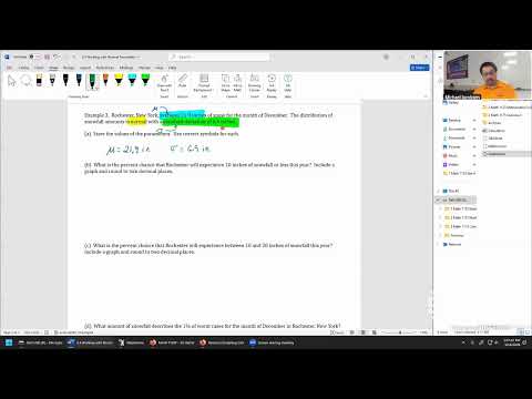
1:05:40 Preview: Rochester December Snowfall Model

The next example models Rochester, New York, December snowfall as normal with mean μ = 21.9 inches and standard deviation σ = 6.5 inches.
Jacobsen explains that stating parameters first helps distinguish the mean from the standard deviation and supports partial credit if later calculator work is consistent.
The class will continue the snowfall problem in the next session before moving on to Chapter 6.

Summary, takeaways, and chapters were generated by AI from the video's transcript and may contain errors. The video belongs to its creator, Mike Jacobsen.