Math 1153 5 October 2026 Sections 5.3, 5.4

Overview

Mike Jacobsen reviews Sections 5.3 and 5.4 on modeling populations with normal distributions, using the empirical 68–95–99.7 rule to estimate areas and inverse cutoffs under bell curves. Through reaction-time data with mean 1.31 seconds and standard deviation 0.42 seconds, and pollutant batches with mean 75 ppm and standard deviation 4.2 ppm, he explains parameters, shading direction, bounds, probability interpretation, and why calculator-based normal probabilities improve on rough empirical-rule estimates.

Key takeaways

A sample mean and sample standard deviation estimate the population parameters mu and sigma, allowing a normal curve to make population-level predictions.
The empirical 68–95–99.7 rule only gives rough probabilities at exact standard-deviation landmarks; for example, 1.73 to 2.57 seconds contains 13.5% + 2.35% = 15.85%.
Shading direction must follow the context: slower reaction times and higher pollutant levels require right-tail shading, while cleaner water requires left-tail shading.
For pollutant batches modeled by mu = 75 ppm and sigma = 4.2 ppm, approximately 16% exceed 79.2 ppm, demonstrating that an average below the legal limit does not ensure every batch is compliant.
The interval from 70.8 to 87.6 ppm contains approximately 83.85% of batches under the empirical-rule approximation.
Changing mu shifts a normal curve horizontally, while changing sigma controls its spread; Section 5.4 uses calculator-based normal probabilities to handle arbitrary cutoffs such as the legal limit of 80 ppm.

Chapters

0:00 Course Schedule, Midterm Timing, and Section 5.3 Objectives

Mike Jacobsen explains that Week 7 is approaching midterms, but Math 1153 has Exams 1, 2, and 3 rather than a separate midterm exam.
Exam 2 is planned for the Monday after midterm week, with section coverage and review materials expected around Friday or Saturday.
Section 5.3 serves as a warm-up for Section 5.4, where calculator-based normal probability calculations will replace rough estimates.

2:30 Estimating Population Parameters from Sample Statistics

A sample mean, written as x-bar or y-bar depending on the textbook convention, estimates the population mean parameter mu.
A sample standard deviation S estimates the population standard deviation sigma.
Once estimates for mu and sigma are available, they define a normal model for making predictions about the entire population.

7:30 The Reaction-Time Normal Model with Mean 1.31 Seconds

Reaction-time data for responding to a brake light are modeled with an estimated mean of 1.31 seconds and standard deviation of 0.42 seconds.
Adding or subtracting 0.42 produces the seven empirical-rule landmarks: 0.05, 0.47, 0.89, 1.31, 1.73, 2.15, and 2.57 seconds.
The normal model is only appropriate when the underlying data are approximately unimodal and symmetric rather than strongly skewed.

12:30 Using the 68–95–99.7 Rule for Intervals and Lower Tails

The percentage of reaction times between 1.73 and 2.57 seconds is found by adding 13.5% and 2.35%, giving 15.85%.
For reaction times below 0.89 seconds, the relevant areas are 0.15%, 2.35%, and 13.5%, totaling 16%.
Percentages and probabilities describe the same area under the normal curve; percentages are decimal probabilities multiplied by 100.

17:30 Upper-Tail Cutoffs and Directional Language

To describe the slowest-reacting 16% of the population, shading proceeds to the right because slower reaction means a larger time value.
The cutoff is 1.73 seconds, so the correct description is reaction times of 1.73 seconds or longer.
A cutoff without its direction, such as saying only 1.73 seconds, is incomplete because the intended region could be either below or above the value.

22:30 Normal Models as Inferential Predictions

The model uses sample summaries to estimate population parameters and then predicts population behavior rather than claiming certainty.
A conclusion such as '1.73 seconds or longer describes the slowest 16%' is only reliable if the sample reasonably fits a normal shape.
Section 5.4 will improve on the empirical rule by calculating areas for values such as 1.00 second or 80 ppm that do not fall exactly on standard-deviation landmarks.

27:30 Pollutant Concentration Scenario: Mean 75 ppm and Legal Limit 80 ppm

A manufacturing process releases treated water containing a chemical pollutant, with a legal maximum of 80 parts per million.
The company tunes its scrubbing machine to produce an average concentration of 75 ppm, but the average alone does not reveal how often batches exceed the legal limit.
The output is assumed to follow a normal model with standard deviation 4.2 ppm.

32:30 Parameters versus Statistics: mu, sigma, x-bar, and S

The population mean is represented by mu, while a sample mean such as x-bar or y-bar is a statistic used to estimate it.
The population standard deviation is sigma, while S denotes the sample standard deviation.
For the pollutant model, the parameters are mu = 75 ppm and sigma = 4.2 ppm, describing all current and future batches under the model.

37:30 Constructing the Pollutant Normal Curve and Empirical Percentages

Starting at the mean of 75 ppm, adding 4.2 gives the right-side landmarks 79.2, 83.4, and 87.6 ppm.
Subtracting 4.2 gives the left-side landmarks 70.8, 66.6, and 62.4 ppm.
The empirical-rule regions are 34%, 13.5%, 2.35%, and 0.15% on each side of the mean, summing to 100%.

42:30 Finding the Cleanest 2.5% of Pollutant Batches

Cleaner water corresponds to lower pollutant concentrations, so the 2.5% cleanest batches are shaded to the left.
The left-tail areas 0.15% and 2.35% combine to 2.5%, stopping at 66.6 ppm.
The correct interpretation is 66.6 ppm or lower, not simply 66.6 ppm, because the shaded region extends leftward.

47:30 Estimating the Probability of Exceeding 79.2 ppm

The proportion of batches above 79.2 ppm is found by adding 13.5%, 2.35%, and 0.15%, producing 16%.
Although the legal threshold is 80 ppm, the empirical rule cannot directly evaluate 80 because 80 is not one of the diagram's standard-deviation landmarks.
The result implies that roughly 16% of batches may exceed 79.2 ppm, showing why a mean of 75 ppm does not guarantee regulatory compliance.

52:30 Between-Boundary Probabilities from 70.8 to 87.6 ppm

The interval from 70.8 to 87.6 ppm includes the central 34% regions, the adjacent 13.5% region, and one 2.35% region.
Adding 34% + 34% + 13.5% + 2.35% gives an estimated probability of 83.85%.
The same result can be obtained by subtracting the excluded tail areas from 100%, illustrating two equivalent area-computation strategies.

57:30 Section 5.4: The Normal Density Function and Calculator Modeling

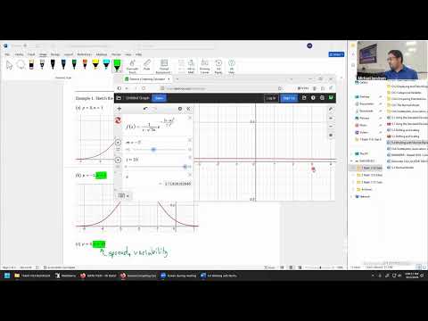
The normal curve is generated by a mathematical density function involving mu and sigma; students are not required to memorize the full formula.
The distribution is unimodal and symmetric, with mu determining the center and sigma determining the spread.
Mike Jacobsen uses Desmos for demonstration only, noting that graphing the density function is not required for quizzes, homework, or MyLab.

1:05:00 How Changing mu and sigma Reshapes a Normal Curve

Changing mu from 0 to -2 shifts the peak horizontally without changing the curve's shape.
Increasing sigma from 1 to 10 spreads the curve across a much wider horizontal range and lowers its apparent peak; axis scaling affects how the curve looks.
A standard deviation must be positive: sigma = 0 collapses the distribution because every observation would be identical, and negative standard deviations are not meaningful.

Summary, takeaways, and chapters were generated by AI from the video's transcript and may contain errors. The video belongs to its creator, Mike Jacobsen.