Math 1153 - 3 September 2026 - Sections 2.2, 2.3

Overview

Mike Jacobsen explains the course’s take-home quiz and exam procedures, then finishes Section 2.2 by teaching how to describe quantitative distributions using modality, symmetry, and skew. He previews Section 2.3’s three-part shape analysis—modes, symmetry or skew, and outliers—and applies it to histograms, including a uniform distribution.

Key takeaways

A quiz earns 10 points, split evenly between submitting work and correctness; the two lowest quiz scores are dropped after the final exam, and quizzes contribute 15% of the course grade.
For a quantitative histogram, count only substantial concentrations as modes: small bar-to-bar fluctuations do not automatically turn a unimodal distribution into a multimodal one.
Skew is named for the direction of the longer tail: unusually long high-value tails indicate right (positive) skew, while long low-value tails indicate left (negative) skew.
Symmetry is judged approximately by comparing the histogram’s two sides around a center line; small samples of roughly 10–20 observations commonly produce imperfect symmetry.
Categorical bar charts have no meaningful distribution shape because rearranging category order can change the chart’s apparent outline.
A useful distribution description covers three features—number of modes, symmetry or skew direction, and outliers—and an observation far from the center is not automatically an outlier if it fits the overall pattern.

Chapters

0:00 Course Schedule, Holiday Break, and First Quiz Announcement

Mike Jacobsen says Monday is a holiday with no class or office hours; the class resumes Tuesday.
The first quiz is posted in Canvas, and Jacobsen previews its format and submission options.

2:00 Finding the Canvas Quiz and Understanding Its One-Problem Format

The quiz appears at the bottom of the Canvas module and includes a broadly compatible PDF plus an optional DOCX file.
Each quiz is typically one scenario with a few parts, based on concepts already covered in class and homework.

4:00 How Weekly Quizzes Preview Exam Questions and Study Guides

Jacobsen says exam questions may reuse quiz problems with changed contexts or altered details.
After grading at the end of Week 3, he plans to post Exam 1’s sections and a study guide with additional practice problems.

6:00 Take-Home Quiz Rules: Open Notes, Open Book, and Instructor Help

These are take-home quizzes, not supervised testing-center assessments; students may use notes, books, and other resources.
Students may ask about quiz problems in class, by email, or during office hours, including before submitting a solution.

10:00 Quiz Submission Formats and the Exam Notes Allowance

Quiz work can be handwritten on notebook paper, printed on the PDF worksheet, or completed digitally with a pen or tablet.
Students submit a scan or photo to Canvas, or may email the work to Jacobsen’s ISU address if needed.
Exams are closed-book with a calculator allowed and one letter-sized sheet of notes, usable on both sides.

14:00 Quiz Scoring, One Attempt, Dropped Scores, and Due-Date Strategy

Each quiz is worth 10 points: 5 points for submitting work and 5 points for correctness; quizzes count for 15% of the course grade.
Quizzes allow one attempt, while MyLab homework allows unlimited retries; Jacobsen will drop the two lowest quiz scores after the final exam.
The first quiz is due September 10, but Jacobsen recommends starting soon after the material is taught to retain it and ask questions before the deadline.

16:30 Reading the Pacific Bluefin Tuna Radioactivity Histogram

The histogram measures Pacific bluefin tuna radioactivity in becquerels per kilogram, grouped into numerical intervals.
Four fish fall in the 6–8 range, one in 8–10, and five in 10–12, illustrating how bar height represents frequency.
Jacobsen identifies the distribution as bimodal because it has two separated concentrations of observations.

18:40 Distinguishing Unimodal and Bimodal Data by Major Peaks

Unimodal data has one major concentration; a small rise in one bar does not necessarily create another mode.
Bimodal data has two substantial, separated clusters, as in the tuna measurements around 6–8 and 10–12.
Jacobsen emphasizes that the gap and renewed concentration help distinguish two modes from a minor fluctuation in a single-mode histogram.

22:20 Multimodal Distributions and Gas-Station Spending Examples

A distribution with three or more major peaks is described as multimodal; Jacobsen also uses trimodal for three peaks.
His hypothetical gas-station histogram has peaks for purchases around $30–$40, $50–$60, and $90–$100.
The separated clusters could reflect drivers with different vehicle sizes, from smaller cars to trucks.

32:00 Symmetric Histograms and the Fold-Over Test

A symmetric histogram has left and right sides that approximately mirror one another around a vertical center line.
The fold-over test checks whether corresponding bar heights roughly overlap; exact symmetry is not required.
Jacobsen notes that real samples of about 10–20 observations often show irregularities, even when the population is expected to be symmetric.

39:30 Right Skew, Long Tails, and Light-Bulb Lifetimes

A unimodal distribution is right-skewed, or positively skewed, when its right tail extends substantially farther than its left tail.
Jacobsen illustrates right skew with LED light-bulb survival times: many bulbs fail in a typical range, while a few last much longer.
The tail’s direction determines the skew label; isolated long-running bulbs extend the distribution to the right.

47:00 Left Skew, Exam Scores, and Why Categorical Data Has No Shape

A left-skewed, or negatively skewed, distribution has a longer lower-value tail; Jacobsen uses a difficult physics exam with many scores from 80 to 100 and fewer low scores.
Modality, symmetry, and skew describe quantitative variables, not categorical data.
Bar-chart category order can be rearranged to change its apparent shape, so a categorical chart must not be called right-skewed or symmetric.

58:00 Section 2.3: A Three-Part Method for Describing Distribution Shape

Jacobsen’s shape checklist asks students to identify the number of modes, assess symmetry or the direction of skew, and check for outliers.
An outlier is an observation that does not fit the pattern of the rest of the data; the 1.5 IQR rule will be introduced later.
At this stage, outliers are identified qualitatively as unusual observations separated from the main data pattern.

1:03:00 Worked Histogram Analysis, Uniform Data, and Upcoming Deadlines

The first Section 2.3 example is unimodal and highly symmetric, with no outliers because its observations follow the overall pattern.
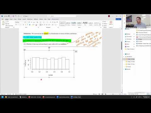
A second histogram is uniform: its bars are roughly the same height, so it has no main peak, yet it can still be symmetric and have no outliers.
Jacobsen plans to resume the second example on Tuesday; Section 2.3 is expected to be due September 15, one week after the section is completed.

Summary, takeaways, and chapters were generated by AI from the video's transcript and may contain errors. The video belongs to its creator, Mike Jacobsen.