Math 1153 - 28 September 2026 - Chapter 4, 5.1

Overview

Mike Jacobsen finishes Chapter 4 by using box plots to compare children’s forced expiratory volume (FEV) across ages and smoking groups, showing how age can explain an apparent smoking–lung-strength paradox. He introduces Chapter 5.1’s z-score formula, applies it to September temperatures and light-bulb lifetimes, and emphasizes that z-scores express distance from the mean in standard deviations.

Key takeaways

A box plot combines the five-number summary with the 1.5-IQR outlier rule; in the example, 184 is flagged because it exceeds the upper fence of 183.75, while the whisker ends at the next non-outlier value, 166.
Grouping FEV measurements by age reveals an increasing median lung-strength pattern and at least eight outliers that are not apparent in the overall histogram.
The apparent higher FEV among children in the smoking group is not evidence that smoking improves lung strength: older age is associated with both greater FEV and higher likelihood of smoking or smoke exposure.
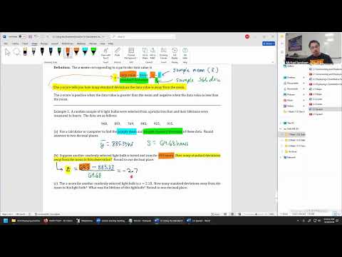
A z-score, z = (y − ȳ)/s, gives both direction and distance from the mean in standard deviations; a positive value is above the mean and a negative value is below it.
With a mean September high of 76°F and standard deviation of 11.1°F, the 91°F September 1 high has z = 1.4, while a hypothetical z = −1.73 corresponds to 56.8°F.
For the six light bulbs, a 693-hour lifetime is 2.7 standard deviations below the 885.33-hour sample mean, marking it as an unusual observation.

Chapters

0:00 Exam 1 Results and the Week’s Chapter 4–5 Plan

Mike Jacobsen reports that Exam 1 has been graded and directs students to the course Grades page for scores and the updating overall course grade.
The class Exam 1 average was 83.2%, with multiple perfect scores.
The lesson finishes Chapter 4 before beginning Chapter 5, Section 5.1.

2:05 Constructing Box Plots with the Five-Number Summary and 1.5-IQR Rule

Begin a box plot with the minimum, first quartile, median, third quartile, and maximum.
Calculate the interquartile range as Q3 − Q1, then flag values below Q1 − 1.5(IQR) or above Q3 + 1.5(IQR) as suspected outliers.
The example’s value of 184 exceeds the upper fence of 183.75, so it is plotted as an outlier; the upper whisker ends at the next non-outlier, 166.

5:29 FEV Data: Lung Strength, Age, Height, and Smoking Status

The study measures children’s forced expiratory volume (FEV), in liters, as an indicator of lung strength, alongside age, height, sex, and smoking exposure.
The overall FEV histogram is slightly right-skewed, with most values around 2–3 liters and a longer upper tail.
A histogram of FEV alone hides how the distribution relates to the study’s other variables.

8:32 Age-Specific Box Plots Reveal FEV Growth and Hidden Outliers

Side-by-side box plots for ages 3 through 19 show median FEV generally rising as children get older, with growth becoming less pronounced in the older age groups.
The age-specific distributions can differ in skew: the 13-year-old group is skewed right, while the 6-year-old group is skewed left.
The combined histogram shows no clearly separated outliers, but the grouped box plots reveal at least eight outlier points across age groups.
Very young groups may have few observations, which can produce box plots with little or no visible whisker.

20:09 Smoking-Group Box Plots Create an Apparent Lung-Strength Paradox

A box-plot comparison of smoking status against FEV appears to show higher lung strength among children in the smoking group, including a higher median.
The smoking indicator includes children who smoke or are regularly exposed to secondhand smoke; zero denotes the non-smoking group.
Jacobsen cautions that this observational comparison does not show that smoking causes higher FEV, and that the pattern is not true for every child.

27:08 Age Is the Lurking Variable Behind the Smoking–FEV Pattern

The data show smoking-group observations more often among older children, while younger children are predominantly in the non-smoking group.
Because FEV tends to increase with age and older children are generally larger, age can explain why the smoking group appears to have higher lung strength.
Age is a lurking variable associated with both smoking status and FEV; the observed association should not be interpreted as a causal effect.
Different relationships in a complex data set may require different displays, such as the scatter plots planned for Chapter 6.

33:20 Chapter 5.1 Introduces Standardization and Z-Scores

Jacobsen frames Chapter 5 as preparation for later normal-distribution and inferential-statistics work, with Sections 5.3 and 5.4 as its larger topics.
Section 5.1 returns to one quantitative variable and uses the sample mean, ȳ, and sample standard deviation, s.
The z-score formula is z = (y − ȳ)/s, where y is an individual data value.

37:33 What a Z-Score Says About a Value’s Distance from the Mean

A z-score counts how many standard deviations a data value lies from the mean.
A positive z-score means the value is above the mean; a negative z-score means it is below the mean.
The sign gives direction, while the absolute value gives the distance in standard-deviation units.

40:21 September Idaho High Temperatures Set Up a Z-Score Example

Jacobsen uses September high temperatures from a 2024 calendar data set, entering the daily highs rather than both highs and lows.
The sample mean is 76°F and the sample standard deviation is 11.1°F.
The mean describes the center of the month’s highs, while the standard deviation provides a scale for judging how unusual an individual high is.

46:53 Recovering a Temperature from a Z-Score of −1.73

A hypothetical September 28 z-score of −1.73 indicates a temperature below the 76°F mean.
Substitute into (y − 76)/11.1 = −1.73 and solve for y; multiplying gives y − 76 = −19.203.
The implied temperature is 56.8°F, rounded to one decimal place.
On a calculator, multiply −1.73 by 11.1, then add 76; the signs in these operations must be opposite.

58:02 Light-Bulb Lifetimes: Calculator Statistics and Z-Score Setup

The next example uses a random sample of six light bulbs, with lifetimes measured in hours.
Jacobsen reviews entering values in calculator list L1 and using STAT → CALC to obtain summary statistics.
The calculator’s x̄ corresponds to the textbook’s sample mean ȳ; use Sx for the sample standard deviation, not the population standard deviation.
The lesson previews using z-scores to compare results across different tests and measurement scales.

1:03:05 A 693-Hour Bulb Lifetime Is 2.7 Standard Deviations Below Average

For the six bulb lifetimes, the sample mean is 885.33 hours and the sample standard deviation is 69.68 hours.
For the bulb lasting 693 hours, z = (693 − 885.33)/69.68, which rounds to −2.7.
The negative sign indicates the bulb’s lifetime is below the sample mean; a distance of 2.7 standard deviations is unusual.
Showing the z-score setup before calculator arithmetic helps preserve work for partial credit and catch entry errors.

1:07:05 Z-Scores Connect Standard Deviation to Typical and Unusual Values

Jacobsen relates one standard deviation from the mean to roughly 68% of data in a suitable distribution and two standard deviations to roughly 95%.
The 693-hour bulb is far from the 885.33-hour center, illustrating how a z-score makes spread comparable in standardized units.
The next class will use z-scores to compare performance across different tests, then move to Section 5.2’s shifting and scaling ideas.

Summary, takeaways, and chapters were generated by AI from the video's transcript and may contain errors. The video belongs to its creator, Mike Jacobsen.