Math 1153 - 27 August 2026 - Chapter 1, Section 2.1
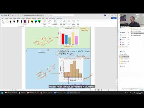 Watch on YouTube →
Overview
Mike Jacobsen introduces variables and data through a Florida lake study of 53 representative lakes, then distinguishes categorical variables from quantitative ones using examples such as zip codes, ISU student credits, and employee project data. He begins Section 2.1 by showing how variable type determines an appropriate display: categorical data use bar or pie charts, while quantitative data use histograms and other ordered displays.
Key takeaways
- A variable’s format alone does not determine its type: zip codes contain digits but are categorical because averaging them has no meaningful interpretation.
- A useful test for a quantitative variable is whether its values have meaningful units and whether an average answers a sensible question.
- In the Florida water-quality dataset, 53 representative lakes form the sample, while all Florida lakes are the population the study aims to learn about.
- Categorical variables call for displays such as bar charts or pie charts; quantitative variables call for ordered displays such as histograms.
- Bar-chart categories can be rearranged, but histogram intervals must remain in numerical order because they represent positions on a measurement scale.
- A histogram bar’s height gives the frequency within its interval: in the cherry-tree example, three trees fall between 65 and 70 feet.
Chapters
0:00
Course Setup and Chapter 1 Progress
- Mike Jacobsen reminds students to open the Pearson MyLab link through Canvas at least once to connect the homework system.
- Chapter 1 is nearly complete; Jacobsen says homework deadlines will move if the class needs extra time to finish a section.
- The class resumes with Example 3 and shifts its focus toward data and variables.
2:43
What Variables and Data Mean in a Statistical Study
- A variable is a characteristic whose value can differ across individuals, such as height or handedness in the blindfolded football-field study.
- The football-field study also measured yards traveled before going off course and whether participants veered left or right.
- Data are observations on one variable or on multiple variables measured together.
4:36
Florida Lakes: Identifying the Sample and Population
- A water-quality study selected 53 representative Florida lakes, making the sample size n = 53.
- The sample is the 53 selected lakes; the population is all lakes in Florida that the study aims to describe.
- The table shows only a few rows of the larger dataset, with ellipses indicating additional lakes through row 53.
9:34
Counting Variables in the Florida Lake Dataset
- The lake table has five variables, one for each column: pH, chlorophyll, average mercury in fish, number of fish sampled, and age of data.
- Mercury is reported in parts per million, and the number of fish sampled explains how researchers estimated each lake’s average.
- Age of data is recorded in categories such as recent or one year old, illustrating that not every variable is numerical.
13:41
Categorical Variables: Groups, Zip Codes, and Age Bands
- A categorical variable assigns individuals to groups; examples include county of residence and blood type for Idaho residents.
- Zip codes and telephone area codes are categorical even though they contain digits: averaging them does not produce a meaningful measurement.
- Age can be categorical when grouped as minor, adult, or senior, but is quantitative when recorded as a numerical age.
21:25
Quantitative Variables: Meaningful Averages and Units
- A quantitative variable records numerical values for which calculating an average makes sense; meaningful units are another useful clue.
- For ISU students registered in fall 2026, examples include number of registered credits and GPA.
- Height and commuting distance can also be quantitative; major, college, and class level are categorical.
31:16
A Company Study Measures Project Completion Time
- A fictional company study investigates factors that may affect how many days employees need to complete a project.
- Researchers select a simple random sample of 10 employees, meaning each employee has an equal chance of selection.
- The table records education, years of experience, communication ratings, workload, and days to complete the project.
36:16
Classifying Employee Variables and Spotting Outliers
- Education, communication rating, and workload are categorical because they sort employees into groups rather than meaningful numerical values.
- Years of experience and days to complete are quantitative: both have units, and averages can be calculated.
- The 78-day completion time and 14 years of experience stand out from the other observations as potential outliers.
41:39
Five Quick Tests for Categorical Versus Quantitative Data
- Potato-chip weight in ounces, grocery items purchased, and gas purchased in gallons are quantitative variables.
- Cola brand is categorical because it groups purchases by brand rather than measuring a numerical amount.
- Gas type—regular, premium, or diesel—is categorical because the possible values are named groups.
49:29
Ceramic Hip Squeaking Is a Categorical Outcome
- The study includes 143 people who received ceramic hip replacements between 2003 and 2005; 10 hips developed squeaking.
- The variable is whether a hip squeaks or does not squeak, so it is categorical rather than a count-based quantitative measurement.
- Identifying the variable type matters because it determines which statistical procedures and formulas are appropriate.
54:22
Section 2.1: Bar Charts and Pie Charts for Categories
- Section 2.1 begins Chapter 2’s focus on displaying and describing data, with display choices guided by whether a variable is categorical or quantitative.
- Pie charts and bar charts are the two main displays introduced for categorical data; the course will focus mostly on bar charts.
- In a favorite-color bar chart, colors are categories, and the bars show how many observations fall into each category.
59:14
Histograms Preserve the Order of Quantitative Measurements
- Histograms are a central display for quantitative data; other options include stem-and-leaf plots, dot plots, and box plots.
- Unlike bar-chart categories such as favorite colors, histogram intervals follow a numerical scale and cannot be rearranged.
- Bar charts typically have gaps between categories, while histogram bars usually touch because the measurement scale is continuous.
1:05:03
Reading Histogram Frequencies for Cherry-Tree Heights
- A histogram of black cherry tree heights uses measurement intervals from about 60 to 90 feet and a vertical frequency scale.
- A bar spanning 65 to 70 feet with height 3 represents three trees in that height interval.
- The histogram makes the distribution’s shape and spread visible, including a concentration around 75–80 feet and fewer trees toward the extremes.
1:08:10
Chapter 2 Preview: From Displays to Numerical Summaries
- Chapter 2 will move from displaying data to describing it with quantities such as minimum, maximum, and average.
- Jacobsen plans to continue with the next example on Monday, after reviewing the difference between bar charts and histograms.
- The course will first emphasize categorical data, then spend the remainder of the chapter on quantitative data and calculations.
Summary, takeaways, and chapters were generated by AI from the video's transcript and may contain errors. The video belongs to its creator, Mike Jacobsen.