Math 1153 - 24 September 2026 - Chapter 4

Overview

Mike Jacobsen teaches how to build and interpret box plots, using a TI calculator to obtain five-number summaries and the 1.5×IQR rule to identify suspected outliers. Examples include radioactive fish measurements and Cornell’s 2003 Christmas Bird Count; the lecture closes by previewing side-by-side box plots for children’s forced expiratory volume (FEV) data.

Key takeaways

For the radioactive-fish data, Q1 = 8, Q3 = 11.8, and IQR = 2.8; the 1.5×IQR cutoffs are 3.8 and 16, so the observed range of 4.6–15.6 contains no suspected outliers.
For the 2003 Christmas Bird Count, the five-number summary is 82, 97.5, 112, 132, and 184 species, with an IQR of 34.5.
The bird-count upper outlier cutoff is 183.75 species, so 184 is a suspected outlier; the lower cutoff is 45.75, well below the minimum of 82.
A box plot’s box spans Q1 to Q3 and contains the central 50% of the data; whiskers extend to the most extreme non-outlier values, while flagged outliers are plotted separately.
The bird-count distribution is right-skewed because its upper tail is more spread out; its median of 112 species is a context-specific measure of a typical site.
Side-by-side box plots help compare a quantitative outcome such as children’s FEV across categories such as age, smoke exposure, and sex, where a single histogram cannot show group differences.

Chapters

0:00 Course Updates and Chapter 4’s Box-Plot Focus

Mike Jacobsen plans to finish grading the week’s exams and publish grades on Canvas by Sunday.
The class is working through Chapter 4 on comparing distributions; Chapter 5 will introduce normal distributions.
Quiz 3 is due that day, and Quiz 4 is already posted.

3:01 TI Calculator Statistics for the Radioactive-Fish Data

The fish data measure radioactivity in becquerels per kilogram, collected off California four months after Japan’s nuclear meltdown.
Jacobsen enters the observations in the TI calculator using STAT, EDIT, then STAT, CALC, 1-Var Stats to obtain summary statistics.
The five-number summary’s minimum and maximum are 4.6 and 15.6; the calculator supplies Q1, the median, and Q3.

10:12 The 1.5×IQR Rule for Flagging Suspected Outliers

An observation is flagged if it exceeds Q3 + 1.5×IQR or falls below Q1 − 1.5×IQR.
Calculate the interquartile range as IQR = Q3 − Q1; it measures the spread of the central 50% of observations.
Jacobsen emphasizes that this is a rule of thumb, not proof: an unusual value may reflect a typo, such as entering 80 instead of 8.0, or a different kind of fish.

13:37 Checking Both Fish-Data Outlier Boundaries

For the fish, Q1 = 8, the median is 10.5, Q3 = 11.8, and IQR = 11.8 − 8 = 2.8 becquerels per kilogram.
The upper cutoff is 11.8 + 1.5(2.8) = 16; the maximum, 15.6, is below it.
The lower cutoff is 8 − 1.5(2.8) = 3.8; the minimum, 4.6, is above it, so neither end contains a suspected outlier.

22:09 Introducing Cornell’s Christmas Bird Count Data

The example uses 2003 counts from 20 sites participating in Cornell Lab of Ornithology’s Christmas Bird Count.
Each observation is the number of bird species recorded at a site; the values range from 82 to 184.
Jacobsen enters the 20 observations into calculator list L1 and recommends checking the entry carefully because a mistyped value affects the statistics.

31:00 Bird-Count Five-Number Summary and IQR

The calculator gives a minimum of 82 species, Q1 = 97.5, median = 112, Q3 = 132, and maximum = 184.
Q1 may be fractional even though species are counted as whole numbers: 97.5 marks a quartile boundary, not a literal half-species observation.
The bird-count IQR is 132 − 97.5 = 34.5 species.

34:10 Bird-Count Outliers at the Upper and Lower Cutoffs

The upper cutoff is Q3 + 1.5×IQR = 132 + 1.5(34.5) = 183.75 species.
The value 184 exceeds 183.75, making it the sole suspected upper outlier and also the maximum.
The lower cutoff is Q1 − 1.5×IQR = 97.5 − 1.5(34.5) = 45.75; since the minimum is 82, there are no lower outliers.

41:08 Choosing a Scale for the Bird-Count Box Plot

Jacobsen draws a vertical axis for number of bird species and chooses a scale from 80 to 200 to include the full 82–184 range.
Tick marks every 20 species provide a readable scale with roughly 5–10 intervals.
A box plot can be oriented horizontally or vertically; the orientation is a stylistic choice.

45:13 Drawing the Box, Whiskers, and 184-Species Outlier

The box spans Q1 = 97.5 to Q3 = 132, with a median line at 112; this interval contains the central 50% of observations.
The lower whisker extends from Q1 down to the minimum of 82.
The 184 value is marked separately as an outlier, while the upper whisker ends at the next-highest non-outlier, 166.

53:20 Reading the Bird-Count Box Plot in Context

A useful interpretation should describe at least three features in context, such as the number of species recorded across the 2003 bird-count sites.
The 184-species observation is a suspected outlier worth checking for possible counting or classification errors.
The box plot also communicates the distribution’s shape, typical value, and spread—not just its five-number summary.

57:39 Identifying Right Skew from Unequal Box-Plot Spacing

The bird-count distribution is skewed right: the upper tail from Q3 toward the high values is more spread out than the lower tail.
For a vertical box plot, right skew appears as a longer extension upward because larger values correspond to the right on a horizontal scale.
Q1, the median, and Q3 mark the 25th, 50th, and 75th percentiles; the box between Q1 and Q3 contains the central 50%.

1:01:01 Using the Median and Box Plots to Compare Groups

The bird-count median is 112 species, a defensible measure of a typical site; visual estimation from the plotted scale may look closer to 110.
Jacobsen notes that box plots become especially useful when comparing a quantitative variable across categories or multiple groups.
A complex dataset can include several variables at once, so a histogram of one quantitative variable may not tell the full story.

1:04:22 Previewing FEV Data on Children’s Lung Function

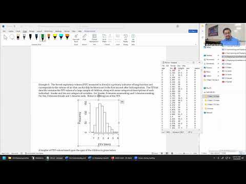
Forced expiratory volume (FEV), measured in liters, records how much air a person can forcefully exhale during the first second after a full breath.
The FEV.txt dataset contains children’s FEV measurements alongside age and categorical variables including smoke exposure and sex.
In the dataset, smoke is coded 0 for non-smoking and 1 for smoking; sex is coded 0 for female and 1 for male.

1:08:35 Next Class: Side-by-Side FEV Box Plots

A histogram summarizes the overall FEV measurements, but side-by-side box plots can compare lung-function distributions across ages and other categories.
The FEV display marks outliers with open circles and illustrates how box plots help analyze mixed quantitative and categorical variables.
Jacobsen plans to continue the example on Monday, then move into Chapter 5 and normal distributions.

Summary, takeaways, and chapters were generated by AI from the video's transcript and may contain errors. The video belongs to its creator, Mike Jacobsen.