Math 1153 - 17 September 2026 - Sections 2.5, Chapter 3

Overview

Mike Jacobsen concludes Section 2.5 by matching measures of center and spread to distribution shape, then applies the median and interquartile range to traffic-congestion cost data for 13 large urban areas. He introduces Chapter 3’s two-way tables using a 626-person tattoo and hepatitis C study, explaining marginal and conditional distributions and calculating that 7.5% of participants had hepatitis C.

Key takeaways

For roughly symmetric quantitative data, pair the sample mean ȳ with standard deviation s; for clearly skewed data, pair the median with IQR.
In the urban traffic-cost example, the right-skewed distribution has a median of $4 million and an IQR of $2.5 million, with two high outliers at $13 million and $15 million.
The IQR equals Q3 − Q1 because Q1 marks the 25th percentile and Q3 the 75th; the interval between them contains approximately the central 50% of observations.
A marginal distribution summarizes one categorical variable for the entire sample, while a conditional distribution restricts the sample to a specified category of the other variable.
In the 626-participant study, 47 had hepatitis C, so the overall sample proportion is 47/626, or 7.5%; a conditional calculation would use a subgroup-specific denominator instead.
An association between tattoo status and hepatitis C in an observational study does not demonstrate that either variable causes the other.

Chapters

0:00 Exam 1 Scope, Calculator Practice, and Testing Reminders

Exam 1 covers Chapter 1 and Sections 2.1–2.3; Section 2.4 is excluded because it was completed recently.
Students may bring one double-sided notes page and must bring a calculator; the Pocatello testing center requires notes in pen or printed.
Quiz 3 is available on Canvas for additional TI-84 calculator practice, and students are asked to schedule Exam 1 promptly.

3:49 Choosing Center and Spread by Distribution Shape

For roughly symmetric distributions, use the sample mean, ȳ, for center and the sample standard deviation, s, for spread.
With severe skew, the mean shifts toward the tail and standard deviation becomes misleading because it is calculated from deviations around the mean.
The median and interquartile range are robust to skew: the median marks the 50th percentile, while IQR describes the central half of observations.

6:03 Reading Skew and Outliers in Urban Traffic-Cost Data

The example uses estimated traffic-congestion costs, in millions of dollars, for 13 large urban areas from a 2015 Urban Mobility Scorecard report discussing 2017 estimates.
The histogram is unimodal and right-skewed, with most observations between $2 million and $4 million.
Two unusually large observations, $13 million and $15 million, appear above $12 million and are identified as outliers.

11:16 Selecting Median and IQR for Right-Skewed Costs

Because the traffic-cost distribution is right-skewed, the appropriate summaries are the median for center and IQR for spread.
Pairing matters: use median with IQR, or sample mean ȳ with sample standard deviation s; do not mix the measures across pairs.
A question asking which statistics to use is asking for names or symbols, not for the statistics to be calculated.

15:32 Finding and Interpreting the Median on a TI-84

Mike Jacobsen enters the 13 urban-area cost values into the TI-84’s statistics list and uses the one-variable statistics calculation.
The calculator reports a median of 4, meaning the middle estimated congestion cost is $4 million.
The interpretation uses the study context and percentile meaning: about half the urban areas fall below the median and half above it.

20:02 Calculating the Traffic-Cost IQR

The IQR is calculated as Q3 − Q1; the example uses Q3 = 6 and Q1 = 3.5, giving an IQR of 2.5 million dollars.
Because the variable measures lost money from traffic congestion, the IQR’s units are millions of dollars.
Interpret the result as the width of the interval containing approximately the central 50% of urban-area costs.

24:03 Why Q1-to-Q3 Covers the Central 50%

Q1 is the 25th percentile and Q3 is the 75th percentile, so roughly 25% of observations lie below Q1 and 25% lie above Q3.
The observations between Q1 and Q3 therefore make up approximately 50% of the data; the median is also called Q2 or the 50th percentile.
For the 13-observation example, three values below Q1 = 3.5 represent about 23% of the data, illustrating why small samples yield approximate rather than exact quartile percentages.

31:19 Chapter 3: Contingency Tables for Two Categorical Variables

Chapter 3 returns to categorical data after Chapter 2’s focus on quantitative variables; the planned coverage is Sections 3.1 and 3.2.
A contingency table, also called a two-way table, organizes counts or percentages across two categorical variables.
Unlike a one-variable frequency table, a two-way table places categories for one variable across rows and the other variable across columns.

36:23 Defining the Tattoo and Hepatitis C Study Variables

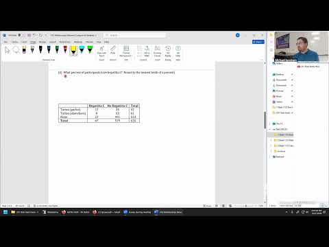
The example describes a University of Texas Southwestern Medical Center study of 626 participants examining whether hepatitis C status was related to tattoo status and where tattoos were obtained.
Mike Jacobsen emphasizes that an observed relationship does not establish causation; another variable could explain an association.
The two categorical variables are tattoo status/location and hepatitis C status; categories such as “tattoo parlor,” “elsewhere,” and “none” are outcomes, not variable names.
Thinking through a raw-data spreadsheet—with one row per participant and columns for tattoo and hepatitis—helps identify the variables hidden by the summarized table.

48:17 Marginal Distributions: Summarizing Each Variable Separately

A two-variable contingency table has two marginal distributions, one for each variable, formed from the row or column totals.
The tattoo marginal distribution is 52 parlor tattoos, 61 tattoos obtained elsewhere, and 513 participants with no tattoos, totaling 626.
The hepatitis C marginal distribution is 47 participants with hepatitis C and 579 without it, also totaling 626.
A marginal distribution ignores the other variable and shows how the full sample is divided among one variable’s categories.

56:01 Conditional Distributions: Restricting to a Given Group

A conditional distribution asks how one variable is distributed after restricting attention to a specified outcome of the other variable.
For tattoo status given no hepatitis C, use only the “no hepatitis C” column: 35 parlor, 53 elsewhere, and 491 with no tattoos.
The conditional total is 579—not 626—because only participants without hepatitis C are included.
The condition identifies which part of the table to use; the remaining variable’s categories and counts form the new distribution.

1:03:00 Calculating the Overall Hepatitis C Percentage

For “what percent of participants have hepatitis C,” “of participants” sets the denominator at all 626 people, while 47 is the hepatitis C count.
Compute 47 ÷ 626 × 100 and round only after converting to a percentage; the result is 7.5% to the nearest tenth.
The example illustrates why a study of a relatively rare condition needs a large sample: only 47 of the 626 participants had hepatitis C.

1:08:31 Exam Week Schedule and Chapter 3 Continuation

The class will not meet on Monday, September 21, when Exam 1 is scheduled.
Mike Jacobsen plans to resume Chapter 3 on Tuesday, September 22, and invites students to email questions.

Summary, takeaways, and chapters were generated by AI from the video's transcript and may contain errors. The video belongs to its creator, Mike Jacobsen.