Math 1153 - 15 September 2026 - Section 2.5

Overview

Mike Jacobsen reviews Section 2.5 statistics, illustrating how the mean and standard deviation describe center and spread for roughly symmetric data, while the median and IQR suit strongly skewed data. He works through a by-hand sample variance and standard deviation for 13, 15, 19, and 21—getting mean 17, variance 13.333, and standard deviation 3.7—then connects the methods to calculator use and exam preparation.

Key takeaways

For the sample 13, 15, 19, and 21, the mean is 17, the squared deviations sum to 40, sample variance is 40 ÷ (4 − 1) = 13.333…, and sample standard deviation rounds to 3.7.
Deviations from the mean sum to zero, so variance measures spread by squaring each deviation before adding them.
Sample variance uses n − 1 in its denominator; with four observations, divide the squared-deviation total by 3.
Use the mean and standard deviation as a pair for roughly symmetric distributions; use the median and IQR = Q3 − Q1 for strongly skewed data or extreme outliers.
Standard deviation is easier to interpret than variance in context because taking the square root restores the original measurement units.
For Exam 1 preparation, Jacobsen recommends setting up the notes page, completing MyLab and Quizzes 1–2, and then practicing with sample exams.

Chapters

0:00 Exam 1 Logistics and the Section 2.5 Review

Mike Jacobsen says the class is finishing Chapter 2 before moving to categorical variables in Chapter 3.
Exam 1 covers the current chapter and three sections; students can bring MyLab, quiz, and sample-exam questions to Thursday's review.
Students should consult Canvas or email Mike Jacobsen for exam-scheduling instructions.

3:09 Interpreting Mean, Standard Deviation, Median, and IQR

In the skin-wound healing example, the sample mean is 25.7 micrometers per hour, while standard deviation describes spread around that mean.
For roughly symmetric data, about 68% of observations fall within one standard deviation of the mean.
The median splits observations in half; Q1 and Q3 mark the 25th and 75th percentiles, so the IQR covers the central 50%.
Mean and standard deviation both summarize center and spread, as do the median and IQR.

8:45 Set Up a Hand Calculation of Sample Mean and Variance

Jacobsen uses four observations—13, 15, 19, and 21—to unpack the sample-statistic formulas before relying on a calculator for later problems.
The sample size is n = 4, and the sample mean is the sum of the observations divided by n.
The values total 68, giving a sample mean of 68 ÷ 4 = 17.
The expanded notation y₁ through yₙ represents each observation; summation means adding all the listed values.

14:43 Calculate Deviations and Square Them to Measure Spread

Subtract the mean 17 from each observation to get deviations −4, −2, 2, and 4.
The deviations always sum to zero, so their unsquared total cannot measure variability.
Squaring the deviations gives 16, 4, 4, and 16, making every contribution nonnegative.
On a TI-84, enter a negative value with the negative-number key and parentheses before squaring; otherwise the result or syntax may be wrong.

24:28 Compute Sample Variance and Fix Calculator Entry Errors

The squared deviations total 40; sample variance divides this sum by n − 1, or 3 for a sample of four.
The sample variance is 40 ÷ 3 = 13.333…, retained to three decimal places as an intermediate value.
Jacobsen demonstrates recalling and editing a prior calculator entry; on some TI-84 versions, use second then enter to bring the last entry back.
The denominator n − 1 is the sample-variance formula's divisor, not the sample size n.

31:03 Take the Square Root to Recover Standard Deviation Units

Sample standard deviation is the square root of sample variance: √13.333… rounds to 3.7.
Variance has squared units—for example, inches squared when measurements are in inches—while standard deviation returns to the original measurement units.
TI-84 models differ in how the square-root function is entered: some require closing a parenthesis, while newer displays place the cursor inside the radical.
Jacobsen presents the hand calculation as a one-time explanation; calculator statistics are more practical for larger datasets.

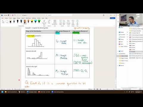
36:09 Match Summary Statistics to Distribution Shape

For roughly symmetric distributions, pair the sample mean (ȳ) for center with sample standard deviation (s) for spread.
For strongly skewed distributions or extreme outliers, use the median (M) for center and IQR = Q3 − Q1 for spread.
Mean and standard deviation belong together because standard deviation measures deviations from the mean; a mean distorted by skew makes that spread measure less useful.
The median and IQR are resistant alternatives that describe the center and central 50% of observations.

42:35 Recognize Center-and-Spread Questions on Exams

A common exam question gives a histogram and asks which statistics best describe center and variability.
Use distribution shape to select the pair: mean and standard deviation for roughly symmetric data, or median and IQR for strong skew.
Jacobsen begins a new, clearly right-skewed dataset but postpones its calculator analysis until the next class.

45:47 Prepare for Exam 1 with Notes, MyLab, Quizzes, and Practice Exams

Start studying by preparing the permitted notes page with useful formulas and definitions from the Canvas sections.
Next, catch up on MyLab homework and Quizzes 1 and 2; Jacobsen accepts late work for full credit.
Use the sample exams after catching up on assigned work, and bring any remaining questions to Thursday's review.
Jacobsen plans to post Quiz 3 before Thursday's class.

Summary, takeaways, and chapters were generated by AI from the video's transcript and may contain errors. The video belongs to its creator, Mike Jacobsen.