Math 1153 - 14 September 2026 - Sections 2.4, 2.5

Overview

Mike Jacobsen reviews Exam 1 logistics and teaches how to choose and calculate statistics for center and spread using a TI-84. He connects distribution shape to mean-versus-median choices, then applies range, sample standard deviation, quartiles, and the interquartile range to data on dementia diagnosis ages and wound-healing rates.

Key takeaways

For roughly symmetric, unimodal data, the sample mean and median are typically close, and the mean is a suitable measure of center; substantial skew makes the median more reliable.
The sample mean follows the long tail: left-skewed data tend to have mean < median, while right-skewed data tend to have mean > median.
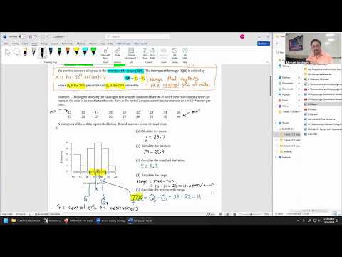
For wound-healing rates, the range is 40 − 11 = 29, whereas the IQR is 33 − 22 = 11 and focuses on the central 50% of observations.
On a TI-84, Sx is the sample standard deviation and σx is the population standard deviation; use Sx by default when observations come from a sample.
For roughly symmetric data, about 68% of observations fall within one standard deviation of the mean; strong skew can make that empirical-rule estimate inappropriate.
Careful TI-84 data entry matters: transposed or duplicated values can alter calculated statistics, so verify L1 entries when outputs disagree.

Chapters

0:00 Exam 1 Scheduling, Coverage, and Allowed Materials

Exam 1 covers Chapter 1 and Sections 2.1–2.3; Mike Jacobsen corrects an initial mistaken reference to Section 2.4.
Students schedule at their indicated testing center, such as Idaho Falls or Pocatello, and should book early because preferred time slots can fill.
Bring a TI-84 calculator and one page of notes, front and back; notes may be handwritten in pen or typed and printed, but not written in pencil.

4:00 Two Exam Review Versions and the Four-Day Testing Window

Version 1 of the Canvas sample exam contains new, section-by-section practice problems and solutions; Version 2 reuses selected lecture-note problems that make suitable exam questions.
The official Exam 1 date is Monday, September 21, 2026, but students may schedule at a testing center from Monday through Thursday, September 21–24.
Monday class is canceled for the exam; scheduling instructions are available through Canvas and the student's ISU email.

9:00 When the Mean or Median Best Describes Center

The mean and median are two measures of center; the median is the 50th percentile, with half the observations below and half above.
For roughly symmetric, unimodal distributions, the sample mean and median are approximately equal, and Jacobsen recommends the mean.
The mean is sensitive to extreme observations, while the median is robust: moving a high outlier far to the right can change the mean substantially while leaving the median near its original value.

15:00 How Left and Right Skew Shift the Mean

The sample mean is pulled in the direction of the distribution's tail: for left skew, mean < median; for right skew, mean > median.
With substantial skew in either direction, the median is the more appropriate measure of center because the mean can be pulled away from the main body of observations.
The stronger the skew or the more influential the outliers, the farther the mean and median can separate.

20:00 Dementia Diagnosis Ages: Identify Skew Before Calculating

The example uses ages at diagnosis for 21 people with early-onset dementia, displayed first as a dot plot and then as a histogram.
The age distribution trails off to the left, so the median is expected to exceed the mean before either statistic is calculated.
The calculated values are a mean of 52.52 years and a median of 54 years, consistent with the left-skew rule.

26:00 Distinguishing the Dementia Sample from Its Population

The sample is the 21 selected people with early-onset dementia whose diagnosis ages were recorded.
The population is all people diagnosed with early-onset dementia, not just the 21 participants.
Jacobsen emphasizes that a good population description preserves the study context and distinguishes the full group from the selected sample.

29:00 Calculate Mean and Median with TI-84 One-Variable Statistics

Open STAT, choose Edit, clear the existing L1 values, and enter the observations carefully; a wrong digit such as 15 instead of 51 can distort the result.
Use STAT, move to CALC, select 1-Var Stats, and specify L1 if the calculator does not default to it.
The calculator labels the sample mean as x̄ and the median as Med; for the dementia data these are 52.52 and 54.

36:00 Range and Variance: Initial Measures of Data Spread

The range is maximum minus minimum, but a single extreme observation can make it a misleading measure of spread.
Jacobsen recalls CEO-to-median-worker pay-ratio data concentrated mostly between 0 and 500, with a large maximum far beyond that cluster.
Variance, standard deviation, and interquartile range offer alternatives that describe spread without relying only on the two endpoints.

48:00 Variance Formula, Standard Deviation, and Quartiles

Sample variance s² sums the squared deviations (y − ȳ)² and divides by n − 1; squaring prevents positive and negative deviations from canceling to zero.
Sample standard deviation s is the square root of s² and is generally used to describe spread when the distribution is roughly symmetric.
Q1 is the 25th percentile, the median is the 50th percentile, and Q3 is the 75th percentile; IQR = Q3 − Q1 captures the central 50% of observations.

54:00 Wound-Healing Data: Compute the Range and Enter Observations

A biology study measures how quickly new cells close small razor cuts on anesthetized newts, in micrometers per hour.
For the supplied data, the maximum is 40 and the minimum is 11, giving a range of 29 micrometers per hour.
Jacobsen recommends clearing L1 and entering the data methodically, then checking calculator results against classmates to catch input errors.

1:01:00 TI-84 Outputs: Mean, Median, Sample Standard Deviation, and IQR

For the wound-healing data, one-variable statistics give a mean of about 25.66 (25.7 to one decimal place) and a median of 26.5 micrometers per hour.
Use Sx for sample standard deviation, about 8.3; the calculator's σx is population standard deviation and is appropriate only when the data represent the entire population.
The calculator supplies Q1 = 22 and Q3 = 33, so the interquartile range is 33 − 22 = 11 micrometers per hour.

1:03:00 Interpret IQR and the 68% Standard-Deviation Rule

The interval from Q1 = 22 to Q3 = 33 contains the central 50% of wound-healing observations, so its width, 11, is a measure of spread around the median.
For roughly symmetric data, about 68% of observations are expected within one sample standard deviation of the mean: approximately 25.7 ± 8.3 for this example.
The empirical rule does not reliably apply to strongly skewed data, while the IQR remains a useful spread measure.

1:08:00 Exam Preparation and Next Class

Jacobsen encourages students to review the posted Exam 1 materials early and bring questions to Thursday's class, which will serve as an open question session.
The next class continues practice with measures of spread before the course moves into Chapter 3.

Summary, takeaways, and chapters were generated by AI from the video's transcript and may contain errors. The video belongs to its creator, Mike Jacobsen.