Math 1153 - 1 October 2026 - Sections 5.2, 5.3

Overview

Mike Jacobsen completes Section 5.2 by showing how a linear transformation, SAT = 40 × ACT + 150, changes measures of position and spread, then introduces normal models in Section 5.3. He explains the 68–95–99.7 empirical rule, how to judge whether data are sufficiently unimodal and roughly symmetric for a normal model, and how to build and interpret a model for driver reaction times with mean 1.31 seconds and standard deviation 0.42 seconds.

Key takeaways

For a transformation SAT = 40 × ACT + 150, measures of position use the full formula, while measures of spread use only the multiplication: an ACT standard deviation of 3 becomes 120 SAT points.
A normal model is appropriate for raw data only when the distribution is unimodal, roughly symmetric, and without obvious outliers; strong skew can make the model misleading.
The empirical rule estimates that 68% of roughly normal observations lie within 1 standard deviation of the mean, 95% within 2, and 99.7% within 3.
A normal model N(μ, σ) uses population parameters: μ is the population mean and σ the population standard deviation; the sample counterparts are y-bar and s.
For driver brake-reaction times modeled as N(1.31, 0.42), the empirical rule estimates that 15.85% of reaction times fall between 1.73 and 2.57 seconds.

Chapters

0:00 Course Announcements and the Shift from Section 5.2 to Normal Models

Mike Jacobsen notes that Quiz 4 is due and Quiz 5 has been posted.
The class finishes the Section 5.2 transformation example before introducing normal models in Section 5.3.
Section 5.3 builds conceptual understanding before calculator-based normal calculations in Section 5.4.

2:20 Reviewing Measures of Position and Spread

Measures of position include the mean, median, quartiles, minimum, and maximum.
The main spread measures used in course problems are sample standard deviation, s, and interquartile range, IQR.
Classifying a statistic as position or spread determines which parts of a transformation formula apply.

5:00 Converting ACT Statistics to SAT Statistics

The example converts statistics from 2,355 students using SAT = 40 × ACT + 150.
The transformation combines rescaling by 40 with a shift of 150.
For measures of position, such as the minimum and mean, apply the entire formula.

10:00 Why Standard Deviation Uses Only the Rescaling Factor

Standard deviation, s, measures spread, so the SAT standard deviation is 40 × 3 = 120 points.
Adding 150 shifts every score but does not change the distance between scores, so it does not affect spread.
The key rule is to use only the rescaling part of a linear transformation for measures of spread.

15:00 Transforming Quartiles, Median, and Interquartile Range

The third quartile is a measure of position, so 40 × 30 + 150 gives an SAT Q3 of 1,350.
The median is also a measure of position: 40 × 28 + 150 gives an SAT median of 1,270.
IQR is a measure of spread, so 40 × 6 gives an SAT IQR of 240 points, with no added 150.

20:00 From Descriptive Statistics to the Normal Model

Descriptive statistics summarize and visualize collected data; inferential statistics use data and models to make claims about a population.
A normal curve can approximate a unimodal, roughly symmetric histogram, but may fit strongly skewed data poorly.
The empirical rule connects the mean and standard deviation to the proportion of observations in different intervals.

22:00 The 68–95–99.7 Rule in Standard-Deviation Units

For unimodal, roughly symmetric data, about 68% of observations fall within one standard deviation of the mean.
About 95% fall within two standard deviations and about 99.7% within three: the 68–95–99.7 rule.
In sample notation, the intervals are centered on y-bar and extend by s, 2s, or 3s in each direction.

29:00 Reading the Normal Curve’s Areas and Tail Percentages

The area between the mean and one standard deviation on each side is about 34%, totaling 68%.
The two bands between one and two standard deviations contribute 13.5% each, bringing the total within two standard deviations to 95%.
The bands between two and three standard deviations contribute 2.35% each; the remaining 0.3% is split into 0.15% in each tail.

34:00 Why Normal Models Require a Shape Check

A normal model is not appropriate for every dataset; the histogram must be unimodal and at least roughly symmetric, with no obvious outliers.
Histograms help assess whether a symmetric bell-shaped curve can reasonably overlay the observed data.
Strong skew can make the sample mean, standard deviation, and normal model inappropriate summaries.

35:00 Applying the Nearly Normal Condition to Histograms

A slight skew may still pass the nearly normal condition if a bell-shaped curve can roughly match the histogram.
A strongly right-skewed distribution fails when a symmetric curve would place substantial area over regions with no observations.
The normal curve must fit both the main peak and the distribution’s overall shape; unimodality alone is not enough.

43:00 Pony Nerve-Cell Counts Versus Traffic-Congestion Losses

A veterinary study counted nerve cells in 23 randomly selected sections of a pony’s intestinal tissue; a suitable model could help characterize the broader region.
Traffic-congestion losses across 13 large U.S. urban areas are strongly right-skewed and therefore do not meet the normal-model shape condition.
The contrast shows why checking histogram shape must come before using a normal curve for inference.

48:00 Population Parameters μ and σ Define a Normal Model

A normal model is written N(μ, σ), where μ is the population mean and σ is the population standard deviation.
These are population parameters, unlike the sample statistics y-bar and s used to describe collected data.
The standard normal model has μ = 0 and σ = 1.

52:00 Modeling Driver Brake-Reaction Times with N(1.31, 0.42)

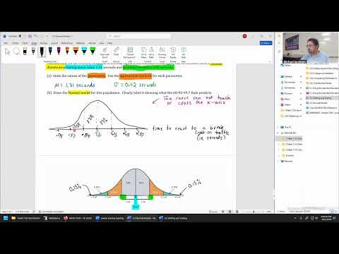
A 1993 study of reaction to standard brake lights reports a normal model with population mean μ = 1.31 seconds and standard deviation σ = 0.42 seconds.
The parameters describe the broader population of drivers, not only the people included in the study.
To sketch the model, label the reaction-time axis and draw a symmetric bell curve that stays above and never touches or crosses the axis.

58:00 Labeling the Reaction-Time Model and Estimating a Population Percentage

Mark the mean at 1.31 seconds and add or subtract 0.42 repeatedly to label the ±1, ±2, and ±3 standard-deviation points: 0.89, 0.47, 0.05 and 1.73, 2.15, 2.57 seconds.
The empirical-rule regions are 34% on each side of the mean, 13.5% in each band from one to two standard deviations, 2.35% in each band from two to three, and 0.15% in each outer tail.
The estimated share of drivers reacting between 1.73 and 2.57 seconds is 13.5% + 2.35% = 15.85%; Jacobsen saves detailed problem-solving for the next class.

Summary, takeaways, and chapters were generated by AI from the video's transcript and may contain errors. The video belongs to its creator, Mike Jacobsen.