Linear Algebra - Lecture 4 - Fall 2026

Overview

Nathanson math lectures reviews subspaces, Gaussian elimination, and solution sets, proving that intersections of subspaces are subspaces and that a homogeneous system with more variables than equations has a nonzero solution. The lecture closes by defining linear combinations, linear dependence, and linear independence, with worked examples in two and three dimensions.

Key takeaways

The intersection of any nonempty family of subspaces is a subspace because zero, vector addition, and scalar multiplication remain valid in every member of the family.
A system’s solution space is a subspace when all equations are homogeneous: each individual solution space is a subspace, and the full solution set is their intersection.
Gaussian elimination preserves solutions through equation swaps, nonzero scalar multiplication, and adding a multiple of one equation to another; a reduced row 0 = 1 signals inconsistency, while 0 = 0 is redundant.
Every homogeneous system with m equations and n variables has a nonzero solution when n > m, as elimination reduces the problem to fewer variables and equations.
The set of all linear combinations of a fixed collection of vectors is a subspace, called their span.
Linear dependence means a nontrivial coefficient choice yields the zero vector; independence means only the all-zero coefficients do so, as demonstrated by the vectors (3, 5) and (1, 2).

Chapters

0:00 Subspaces: The Three Closure Conditions

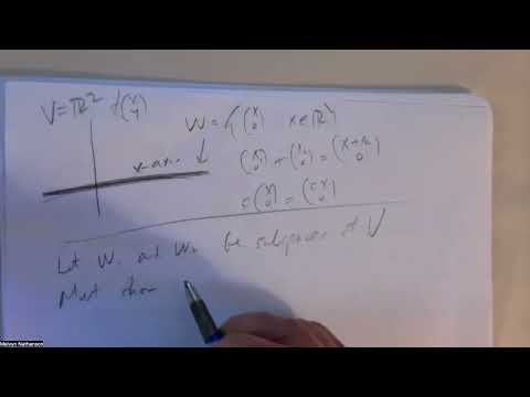
A subspace W of a vector space V must contain the zero vector.
W must be closed under vector addition: if v₁ and v₂ are in W, then v₁ + v₂ is in W.
W must be closed under scalar multiplication: for any real c and v in W, cv remains in W.
The x-axis in ℝ², consisting of vectors (x, 0), illustrates all three conditions.

6:40 Why Intersections of Subspaces Are Subspaces

For subspaces W₁ and W₂, their intersection contains the zero vector because zero belongs to each subspace.
If v₁ and v₂ belong to W₁ ∩ W₂, closure in both W₁ and W₂ puts v₁ + v₂ in the intersection.
For v in W₁ ∩ W₂ and any real c, both subspaces contain cv, so the intersection is closed under scalar multiplication.
The same element-by-element argument works for any nonempty family of subspaces, including infinitely many.

11:30 Solution Spaces of Homogeneous Systems

A homogeneous linear equation has right-hand side zero; its solution space is a subspace.
For a system of two homogeneous equations, define W₁ and W₂ as the individual equation solution spaces.
The system’s solution space is W₁ ∩ W₂, so the intersection result proves it is a subspace.
The argument extends to systems with any number of homogeneous equations.

16:00 The Three Equivalence-Preserving Equation Operations

Two systems are equivalent when they have the same solution set and the same number of variables.
Interchanging equations preserves solutions because it only changes their order.
Multiplying an equation by a nonzero scalar preserves its meaning; for example, x + 2y = 3 is equivalent to 10x + 20y = 30.
Adding a scalar multiple of one equation to another preserves the solution set and forms the basis of Gaussian elimination.

21:00 Gaussian Elimination: A Target Form for Solving

Gaussian elimination uses equivalent equation operations to create a simpler system.
A system with leading coefficients of 1 and zeros in the other entries of each pivot column is especially easy to solve.
In the example with variables x, y, z, and w, w is free and the other variables are expressed in terms of it.
The resulting solution set is an affine subspace: one particular solution plus scalar multiples of a direction vector.

25:00 Worked Elimination for a Two-Equation System

For 2x + y + z = 9 and x + 2y − z = 3, the equations are first interchanged to put a leading 1 on x.
Subtracting twice the first equation from the second eliminates x; dividing the result by −3 gives y − z = −1.
Eliminating y from the first equation gives x + z = 5, so z is free.
The solution is (x, y, z) = (5, −1, 0) + z(−1, 1, 1); substitution checks the particular and direction vectors.

34:00 Clarifying Equation Operations and Their Purpose

A student asks how subtracting twice one equation eliminates the 2x term in the other.
Multiplying x + 2y − z = 3 by −2 and adding it to 2x + y + z = 9 yields −3y + 3z = 3.
Dividing by −3 normalizes the y coefficient to 1, making the resulting system easier to solve.
The instructor stresses that each step is an equivalent-system operation, not an approximation.

38:00 Three Equations in Three Variables: Detecting Redundancy

For x + 4y + 3z = 2, 2x + y + z = 3, and 3x − 2y − z = 4, eliminate x from the second and third equations.
The reduced equations are −7y − 5z = −1 and −10y − 7z = −2.
The third reduced equation is twice the second, so their difference is 0 = 0 and one equation is redundant.
After solving, the system has (x, y, z) = (10/7, 1/7, 0) + z(−1/7, −5/7, 1).

47:00 Contradictions, Redundant Equations, and Inconsistency

A reduced equation 0 = 0 is always true and can be omitted without changing the solution set.
A reduced equation such as 0 = 1 is impossible and proves that the original system has no solution.
The student connects this contradiction test to a second exercise involving three equations in three variables.
The instructor identifies 0 = 1 as evidence that the starting system is inconsistent.

50:00 Comparing Two Systems by Their Solution Sets

The system 7x − 2y = 10 and 3x + y = 21 has the unique solution (x, y) = (4, 9).
A second system adds 4x + 11y = 115 and 8x − 5y = −3 to the equation x + 7y = 67.
Solving the first two equations of the second system gives (4, 9), which also satisfies its third equation.
Because both systems have exactly the same solution, they are equivalent by definition.

56:00 The More-Variables-Than-Equations Theorem

The lecture turns to homogeneous systems with m equations and n variables, focusing on n > m.
Every homogeneous system has the trivial solution with all variables equal to zero.
The theorem states that when n is greater than m, there must also be a nonzero solution.
Examples include one equation in two variables and two equations in three variables.

1:02:00 Proof Base Case: One Homogeneous Equation

For one equation in n ≥ 2 variables, consider whether the coefficient a₁ of x₁ is zero.
If a₁ = 0, setting x₁ = 1 and all other variables to zero directly gives a nonzero solution.
If a₁ ≠ 0, set x₂ through xₙ equal to 1 and choose x₁ = −(a₂ + ⋯ + aₙ)/a₁.
The chosen x₁ may be zero or nonzero; the solution is still nonzero because at least one of x₂ through xₙ equals 1.

1:08:00 Proof for Two Equations by Eliminating a Variable

For two equations in n ≥ 3 variables, if both coefficients of x₁ are zero, setting x₁ = 1 and the remaining variables to zero works.
Otherwise, interchange equations if needed so the first equation has a₁₁ ≠ 0.
Add −a₂₁/a₁₁ times the first equation to the second to eliminate x₁.
The remaining equation has n − 1 ≥ 2 variables, so the one-equation case supplies a nonzero solution that can be extended by solving for x₁.

1:15:00 Induction Proof for m Equations in n Variables

Assume the theorem holds for systems with n − 1 variables and consider m equations with n > m.
If every equation has zero coefficient on x₁, choosing x₁ = 1 and all other variables zero solves the system.
Otherwise, reorder equations to obtain a₁₁ ≠ 0 and eliminate x₁ from each of the other m − 1 equations.
The reduced system has m − 1 equations and n − 1 variables, with n − 1 > m − 1; induction gives a nonzero solution, which extends to the original system.

1:21:00 Linear Combinations Generate Subspaces

A linear combination of vectors v₁, …, vₙ has the form c₁v₁ + ⋯ + cₙvₙ.
The set of all linear combinations of a fixed collection of vectors is closed under addition and scalar multiplication.
That set also contains the zero vector, obtained by choosing every coefficient cᵢ = 0.
Consequently, the span of any collection of vectors is a subspace of the ambient vector space.

1:25:00 Linear Dependence: A Nontrivial Combination Gives Zero

Vectors v₁ through vₖ are linearly dependent if some coefficients, not all zero, satisfy c₁v₁ + ⋯ + cₖvₖ = 0.
The lecture demonstrates dependence with three vectors and coefficients 4, 3, and −1.
The weighted vectors cancel coordinate by coordinate, producing the zero vector despite the coefficients not all being zero.
A nontrivial zero-producing combination distinguishes dependence from the trivial choice in which every coefficient is zero.

1:29:00 Linear Independence: Only the Trivial Combination Gives Zero

Vectors are linearly independent when a linear combination equals zero only if every coefficient is zero.
For vectors (3, 5) and (1, 2), the equation c₁(3, 5) + c₂(1, 2) = (0, 0) becomes 3c₁ + c₂ = 0 and 5c₁ + 2c₂ = 0.
The two-equation system has the unique solution c₁ = c₂ = 0, proving these vectors are independent.
Nathanson math lectures identifies dependence and independence as central concepts for the rest of the linear algebra course.

1:31:00 Lecture Recap: Elimination, Dimension, and Independence

The lecture reviews homework problems on systems of equations and Gaussian elimination.
Its central theorem guarantees a nonzero solution for every homogeneous system with more variables than equations.
Linear combinations, dependence, and independence are introduced as ideas to develop further in the next lecture.
Nathanson math lectures recommends working through proofs carefully and bringing questions to the next class or online office hours.

Summary, takeaways, and chapters were generated by AI from the video's transcript and may contain errors. The video belongs to its creator, Nathanson math lectures.