lecture 9 9

Overview

The lecture develops forward kinematics for a revolute–prismatic robot, including a frame-translation workaround when standard coordinate-frame rules cannot all be met, and derives end-effector position and velocity. It then connects a planar two-revolute-arm velocity model to the Jacobian matrix before demonstrating Dobot Lab controls, coordinate conventions, reach limits, and joint interlocks on the Dobot Magician Lite.

Key takeaways

When a prismatic-joint configuration prevents Xₙ from intersecting Zₙ₋₁, the frame can be translated to the valid intersection; the translation must then be included in the homogeneous-transform displacement.
For the revolute–prismatic example, the end-effector position is pₓ = (A₂ + D) cos θ₁, pᵧ = (A₂ + D) sin θ₁, and p_z = A₁, separating fixed geometry from changing joint variables.
Differentiating position expressions with time-varying joint values requires both chain and product rules; the resulting velocities include Ḋ and θ̇₁ terms, while the constant height A₁ gives ṗ_z = 0.
The Jacobian maps joint speeds to Cartesian end-effector speed, and its configuration-dependent sine and cosine entries mean constant motor speeds can still produce changing tool speeds.
Dobot Lab’s virtual robot reports approximately (240, 0, 145) mm at the demonstrated home pose; matching the simulation’s positive X-forward, Y-left, Z-up axes is essential for valid kinematics.
Robot workspace is constrained by physical joint limits and safety interlocks, so mathematically valid Cartesian targets may still be unreachable on the Dobot Magician Lite.

Chapters

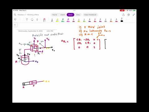
0:00 Revolute–Prismatic Robot: Establishing the Kinematic Diagram

The example combines a revolute joint with a prismatic piston-cylinder assembly and an end effector.
The first setup task is assigning frames so each joint axis is represented by a Z-axis.
The lecture aims to derive the robot’s forward kinematics from its joint variables.

5:00 Handling a Prismatic Joint That Breaks the Frame-Intersection Rule

The usual frame rule requires Xₙ to intersect Zₙ₋₁, but the selected X₁ cannot intersect Z₀ in this geometry.
For this revolute–prismatic arrangement, the lecture allows the intersection rule to be violated temporarily while preserving the joint-axis and right-handed-frame requirements.
A consistent choice of X₁ and the remaining axes completes right-handed coordinate triads.

11:00 Building the First Rotation Matrix with a Nonidentity Projection

The first joint variable is θ₁, and the revolute rotation matrix uses the standard sine-and-cosine form.
Because the selected frame axes are not aligned, the projection matrix is not the identity matrix.
The rotation between frames must be calculated by multiplying the revolute rotation matrix by the projection matrix.

13:00 Translating Frame 1 to Restore the X–Z Intersection

The original frame 1 sits at the prismatic joint, where X₁ remains offset from Z₀.
Translating frame 1 to the point where the axes intersect makes the frame-intersection rule hold.
This translation changes the positional bookkeeping used in the homogeneous transform, not the rotation matrix itself.

18:00 Converting the Adjusted Frame Orientation into a Homogeneous Transform

The projection calculation produces a rotation matrix different from the standard Z-axis rotation matrix because the frame axes are permuted.
The first homogeneous transformation combines this adjusted rotation with the frame-to-frame translation.
The fixed offset A₁ lies along Z₀, with zero translation along X₀ and Y₀.

22:00 Locating the End-Effector Frame After the Prismatic Joint

Frame 2 is placed at the end effector, while frame 1 is the translated frame used to satisfy the intersection rule.
A prismatic joint changes position but introduces no rotation, so the relative rotation from frame 1 to frame 2 is the identity.
The axes of frames 1 and 2 are aligned in this example, making their projection matrix the identity as well.

29:00 Encoding the A₂ Offset and Prismatic Extension

The second homogeneous transform records the separation between translated frame 1 and the original end-effector frame.
That displacement is A₂ + D along the selected frame-1 axis, where D is the prismatic extension.
The first transform’s A₁ offset and the second transform’s A₂ + D displacement are combined by multiplying the two 4×4 matrices.

36:00 Multiplying the Two Transforms to Obtain Frame 2 in Frame 0

The matrix product ⁰H₂ = ⁰H₁ · ¹H₂ gives both the end-effector orientation and position relative to the base frame.
The lecture works through the 4×4 multiplication entry by entry, including the sine-and-cosine terms in the position column.
The final column identifies the end-effector coordinates along X₀, Y₀, and Z₀.

42:00 Checking the Revolute–Prismatic Position Against Robot Geometry

The end-effector position is presented as pₓ = (A₂ + D) cos θ₁, pᵧ = (A₂ + D) sin θ₁, and p_z = A₁.
When D = 0, the end effector lies at radius A₂; extending the prismatic joint increases the radial distance.
The geometric sketch serves as a check on the transformation-based forward-kinematics result.

47:00 Forward-Kinematics Workflow and Coordinate-Frame Rules

Draw a kinematic diagram, align each Z-axis with its joint axis, and form right-handed X–Y–Z triads.
For a revolute joint, use a rotation matrix and multiply by the projection matrix when adjacent frame axes are not aligned.
If the intersection rule fails for a prismatic configuration, translate the frame to the valid intersection and account for that shift in the homogeneous transform.

53:00 Identifying Constants and Time-Varying Joint Variables

In pₓ = (A₂ + D) cos θ₁, A₂ is fixed while D and θ₁ can vary with time.
The corresponding planar position expression also makes pᵧ dependent on both D(t) and θ₁(t).
Time is the independent variable; the joint displacement and joint angle are time-dependent variables.

57:00 Differentiating the X Position with the Chain and Product Rules

Velocity is obtained by differentiating pₓ(t) with respect to time.
The derivative includes the chain-rule term from cos θ₁(t), introducing θ̇₁.
Because D(t) and cos θ₁(t) are both variable, the product rule adds terms involving Ḋ cos θ₁ and −D sin θ₁ θ̇₁.

1:06:00 Finding Y and Z Velocities for the Revolute–Prismatic Robot

Differentiating pᵧ(t) applies the product rule to D(t) sin θ₁(t), yielding terms involving Ḋ and θ̇₁.
The fixed height p_z = A₁ has zero velocity because A₁ is constant.
For robots with more degrees of freedom, the lecture recommends using MATLAB to handle longer derivative expressions.

1:12:00 Position Equations for a Planar Two-Revolute Robot

The next example uses two revolute joints, θ₁ and θ₂, with link offsets including A₂ and A₄.
Its planar position follows pₓ = A₂ cos θ₁ + A₄ cos(θ₁ + θ₂) and pᵧ = A₂ sin θ₁ + A₄ sin(θ₁ + θ₂).
Taking time derivatives converts the joint motions into end-effector velocity components.

1:17:00 Differentiating the Two-Link Position Equations

The derivatives of the combined angle θ₁ + θ₂ contain both θ̇₁ and θ̇₂.
Collecting like terms separates the contribution of each joint velocity to ṗₓ and ṗᵧ.
For this planar example, ṗ_z is zero because the modeled end-effector position has no changing Z component.

1:20:00 Assembling the Two-Revolute Robot’s Jacobian Matrix

The velocity equations are organized as [ṗₓ, ṗᵧ, ṗ_z]ᵀ = J[θ̇₁, θ̇₂]ᵀ.
The first Jacobian row is [−A₂ sin θ₁ − A₄ sin(θ₁ + θ₂), −A₄ sin(θ₁ + θ₂)].
The second row is [A₂ cos θ₁ + A₄ cos(θ₁ + θ₂), A₄ cos(θ₁ + θ₂)]; the modeled third row is zero.

1:25:00 Using the Jacobian to Relate Motor and End-Effector Speeds

Joint velocities θ̇₁ and θ̇₂ correspond to motor speeds, while ṗₓ, ṗᵧ, and ṗ_z describe end-effector velocity.
The Jacobian maps joint velocity to end-effector velocity and varies with the robot’s current joint configuration.
Applications such as painting, welding, pick-and-place, and 3D printing require end-effector speeds to be controlled through the joint motors.

1:27:00 Why Constant Motor Speed Does Not Guarantee Constant Tool Speed

The Jacobian’s sine and cosine terms represent configuration-dependent lever-arm projections.
Even if a motor runs at constant speed, the end-effector velocity can change as the robot’s angles change.
Precise Cartesian motion therefore requires accounting for both motor speeds and the instantaneous Jacobian.

1:31:00 Introducing Dobot Lab and the Dobot Magician Lite

Dobot Lab provides a virtual simulation and can be used through a web version or downloaded for Windows.
The planned lab work uses the Dobot Magician Lite for forward and inverse kinematics.
Dobot Link connects software to a virtual or physical robot using serial communication.

1:37:00 Setting Dobot Lab Coordinates and Connecting the Virtual Robot

The demonstration starts Dobot Link, selects virtual serial port VSP1, and confirms the software connection.
The Dobot’s displayed Cartesian convention is positive X forward, positive Y to the left, and positive Z upward.
The kinematic diagram must use the same axis directions as the physical robot or simulation; flipped axes produce incorrect results.

1:42:00 Reading Dobot Magician Lite Joint and Cartesian Controls

The control panel provides positive and negative controls for joints J1 through J4; joint controls change the end-effector’s Cartesian position.
At the shown home configuration, the lecture reports an end-effector position of approximately X = 240 mm, Y = 0 mm, and Z = 145 mm.
Forward kinematics maps joint values to X, Y, and Z; inverse kinematics finds joint values for a requested Cartesian position.

1:47:00 Dobot Joint Directions, Reach Limits, and Safety Interlocks

The joint axes are identified by observing positive rotations; the demonstrated arm configuration includes a revolute axis perpendicular to another and a further parallel axis.
A mathematically specified X, Y, or Z target may be unreachable because physical joints have limits and the robot has dead zones.
The Dobot Magician Lite includes joint interlocks for safety; changing one joint can automatically affect another, unlike the comparison Dobot Magician described in class.

Summary, takeaways, and chapters were generated by AI from the video's transcript and may contain errors. The video belongs to its creator, ssredkar.