Lecture 9 23

Overview

The lecture develops forward kinematics for the three-joint Dobot Magician Lite by assigning coordinate frames, estimating link dimensions, and composing homogeneous transformations in MATLAB. It then compares calculated end-effector positions with the Dobot Lab simulator, showing that initial estimates of A1 = 45 mm, A2 = 100 mm, and A3 = 240 mm produce reasonable results for some poses but require calibration; inverse kinematics is briefly revisited at the end.

Key takeaways

For the Dobot Magician Lite, assign each frame with its Z axis along a revolute joint, select common perpendicular X axes, and use the right-hand rule to establish the remaining axis directions.
The lecture’s starting dimensions—A1 = 45 mm, A2 = 100 mm, and A3 = 240 mm—are estimates, not verified robot measurements, so agreement at one pose does not validate the whole model.
A link offset must be expressed in the preceding coordinate frame: the A2 displacement becomes −A2 sin(θ2) along X1 and A2 cos(θ2) along Y1 in the illustrated convention.
The forward model composes 0H3 = 0H1 × 1H2 × 2H3, reads px, py, and pz from the final matrix’s fourth column, and includes J2–J3 coupling through θ3 − θ2.
The J1 = 40° test closely matches the simulator, but J2 = 15° produces an approximately 14 mm X discrepancy, demonstrating why validation across multiple joint configurations is essential.
Inverse kinematics cannot reliably reproduce a target pose when the underlying forward-kinematics geometry is miscalibrated; CAD dimensions and physical offsets should be corrected first.

Chapters

0:00 Dobot Magician Lite Kinematics: Goals and Joint Layout

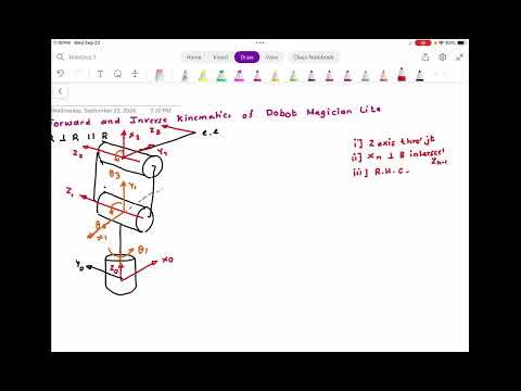
The task is to derive forward and inverse kinematics for the three-joint Dobot Magician Lite.
The first revolute joint is perpendicular to the second, while the second and third joint axes are parallel.
The class plans to use MATLAB and verify results with the Dobot Lab simulator.

1:30 Assigning Joint Axes and Coordinate Frames

The frames are labeled 0 through 3, with Z axes placed along the corresponding revolute joint axes.
The joint variables are named θ1, θ2, and θ3, and their positive directions are checked with the right-hand rule.
A right-handed frame requires the remaining X and Y axes to follow consistently from the selected Z axes.

4:00 Choosing Common Perpendiculars for the Dobot Frames

Each X axis is selected to be perpendicular to and intersect the relevant adjacent Z axis, following the frame-assignment rules.
The frame-1 X axis has a directional choice; the example selects one convenient direction and determines Y1 from the right-hand rule.
The initial X3 placement is corrected so that X3 is perpendicular to and intersects Z2.

10:30 Estimating Link Dimensions from Robot Geometry

The lecture labels the frame-to-frame link distances A1, A2, and A3.
The example uses estimates A1 = 45 mm, A2 = 100 mm, and A3 = 240 mm rather than confirmed physical dimensions.
The physical robot may contain X, Y, and Z offsets that are not represented by a simplified kinematic diagram.

18:00 Building the Base-to-First-Joint Transformation

The 0-to-1 rotation is formed from a rotation about Z0 by θ1 and a projection relating the new and old frame axes.
The homogeneous transform 0H1 combines that orientation with the frame-0-to-frame-1 displacement.
The translation components are interpreted in the original frame, rather than as distances in an unrelated global direction.

22:00 Expressing the Second-Link Offset in Frame 1

The 1-to-2 rotation uses θ2 and the selected axis projections between frames 1 and 2.
When θ2 = 0, the A2 displacement lies along positive Y1; as θ2 changes, it resolves into components along X1 and Y1.
For the illustrated positive-angle convention, the displacement components are −A2 sin(θ2) along X1 and A2 cos(θ2) along Y1.

29:00 Modeling the Third Joint and J2–J3 Coupling

The 2-to-3 transform represents the A3 link with angle-dependent displacement components in the frame-2 directions.
The lecture modifies the third-joint terms to account for mechanical coupling between J2 and J3, using θ3 − θ2.
The complete forward transform is composed as 0H3 = 0H1 × 1H2 × 2H3.

35:00 Extracting End-Effector Position from 0H3

The final homogeneous matrix contains both the end-effector orientation and position.
Position is read from the fourth column: rows 1, 2, and 3 give px, py, and pz.
MATLAB is used to multiply and simplify the transformations because the symbolic expressions are cumbersome to work through by hand.

37:00 Entering the Transform Equations in MATLAB

The 0H1, 1H2, and 2H3 matrices are entered in MATLAB, including the θ3 − θ2 coupling terms.
The equations for px, py, and pz are extracted from the resulting 0H3 matrix.
The initial test uses the assumed link lengths A1 = 45 mm, A2 = 100 mm, and A3 = 240 mm.

44:00 Checking the Model at Zero and J1 = 40°

At θ1 = θ2 = θ3 = 0, the model predicts px = 240 mm, py = 0, and pz = 145 mm.
With J1 set to 40°, MATLAB predicts approximately px = 183.85 mm and py = 154 mm, with pz unchanged.
The Dobot Lab comparison gives approximately x = 183.8 mm at J1 = 40°, providing a close check for this pose.

55:00 Using J2 and J3 Tests to Diagnose Geometry Errors

At J2 = 5°, the model predicts x ≈ 253.3 mm and z ≈ 144.41 mm, while the simulator gives an x position around 248 mm and a similar z value.
At J2 = 15°, the model predicts x ≈ 265 mm and z ≈ 141 mm, compared with simulator values around x = 279 mm and z = 139 mm.
A J3 = 30° comparison also shows a substantial Z discrepancy; the growing pose-dependent error indicates that the assumed link dimensions or offsets need calibration against CAD geometry.

1:01:00 Inverse Kinematics Depends on an Accurate Forward Model

The inverse-kinematics code is used to solve for θ1, θ2, and θ3 from a desired end-effector position.
The returned pose does not match reliably because the forward model still contains link-dimension and offset errors.
The lecture’s practical conclusion is to refine the geometry using CAD measurements and repeat simulator checks before trusting inverse-kinematics results.

Summary, takeaways, and chapters were generated by AI from the video's transcript and may contain errors. The video belongs to its creator, ssredkar.