Lecture 7: Multivariate calculus

Overview

Burton Ma introduces the multivariate calculus notation needed for high-dimensional optimization, including column vectors, vector-valued functions, scalar-valued functions of vectors, partial derivatives, and directional derivatives. He connects the material to deep neural networks with billions of parameters and demonstrates MATLAB implementations for lines, vector norms, and direction-based calculations before defining the gradient as a column vector.

Key takeaways

High-dimensional optimization requires vector calculus because modern deep neural networks may optimize billions of parameters simultaneously.
A vector-valued function of a scalar input is differentiated component by component, so an m-dimensional output produces m ordinary derivatives.
A scalar-valued function of an n-dimensional vector has n partial derivatives, each obtained by varying one coordinate while holding the remaining n - 1 coordinates constant.
The directional derivative along a unit vector v-hat is the dot product of the gradient and v-hat, combining all coordinate-wise partial derivatives according to the chosen direction.
The Euclidean norm of a vector can be represented equivalently as the square root of summed squared components, sqrt(w-transpose w), or MATLAB's norm(w).
Burton Ma uses column vectors for gradients, whereas the course notes use row vectors for the related total derivative, making transpose conventions important in later matrix calculations.

Chapters

0:00 Why Vector Calculus Matters for Billion-Parameter Optimization

Burton Ma transitions from one-dimensional calculus to vector calculus for higher-dimensional optimization problems.
Deep neural networks can contain billions of parameters, creating billion-dimensional optimization problems that require generalized calculus techniques.
The course uses an arrow above symbols to distinguish vector quantities from scalar and matrix quantities.
Vectors are represented by default as n-dimensional column vectors with components w1 through wn; row vectors are obtained through transposition.

4:00 Vector-Valued Functions and Parametric Lines in MATLAB

A vector-valued function maps a scalar t to an m-dimensional vector, with each component represented by a scalar function such as f1(t) through fm(t).
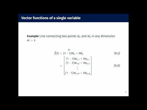
A line through points wa and wb is parameterized as (1 - t)wa + twb, giving wa at t = 0, wb at t = 1, and points beyond the segment for other real values of t.
Burton Ma implements the line formula in MATLAB and uses element-wise dot notation when t is an array of 101 values from -1 to 1.
MATLAB stores the evaluated line points as a matrix whose columns represent individual points and whose rows contain coordinates such as x and y.

12:00 Unit-Direction Lines, Vector Norms, and a 3D Helix

A line can also be written as a point a plus a scalar t multiplied by a unit direction vector d-hat.
MATLAB's norm function computes the L2 norm, corresponding to the Euclidean length obtained from the square root of summed squared components.
A direction vector is normalized by dividing it by its norm; choosing direction wb - wa reproduces the line through two points.
A three-dimensional helix is represented parametrically with cosine and sine coordinates plus a linearly increasing z-coordinate.

15:00 Derivatives of Vector-Valued Functions

The derivative definition for a vector-valued function uses the same limit, [f(t + h) - f(t)] / h, as the scalar case.
Differentiating a vector function of a scalar input reduces to differentiating each component function independently.
For an m-dimensional output, the derivative produces m scalar derivatives corresponding to the component functions f1(t) through fm(t).
The result applies directly to parametric curves such as the previously defined line and helix.

17:00 Scalar Functions of Vectors and Partial Derivatives

A scalar-valued function of a vector maps w in R^n to a real number; the Euclidean length ||w|| is a central example.
Vector length can be written as the square root of summed squared components, the square root of w-transpose times w, or MATLAB's norm(w).
To define a derivative with respect to one component, all other components are held constant; this produces a partial derivative.
For f(x, y) = x^2 + y^2, holding y fixed gives partial f/partial x = 2x, while holding x fixed gives partial f/partial y = 2y.

24:00 Standard Basis Vectors, Directional Derivatives, and the Gradient

The standard basis vectors e1 through en generalize the familiar i-hat, j-hat, and k-hat vectors to R^n; each contains one 1 and zeros elsewhere.
A partial derivative can be expressed using the limit [f(w + h e_j) - f(w)] / h, where e_j changes only the jth input coordinate.
Replacing e_j with an arbitrary unit vector v-hat defines the directional derivative of f at w in the direction v-hat.
The directional derivative equals the sum of each partial derivative multiplied by the corresponding component of v-hat, or equivalently the dot product of the gradient with v-hat.
Burton Ma defines the gradient as the column vector of partial derivatives, while noting that the course notes use a row-vector convention associated with the total derivative.

Summary, takeaways, and chapters were generated by AI from the video's transcript and may contain errors. The video belongs to its creator, Burton Ma.