Lecture 6: Armijo condition
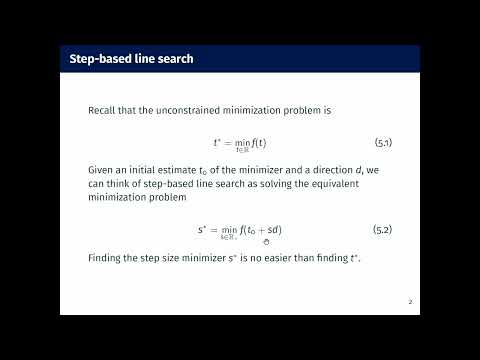 Watch on YouTube →
Overview
Burton Ma explains why a fixed step size can diverge or fail to converge, then derives the Armijo sufficient-decrease condition from a first-order Taylor approximation. He shows how backtracking tests successively smaller step sizes, demonstrates its use in MATLAB, and briefly contrasts Armijo with the stronger Wolfe conditions.
Key takeaways
- For a quadratic objective with negative-gradient updates, tₖ₊₁ = (1 − s)tₖ, so fixed step sizes that are too large can cause divergence while smaller ones may converge slowly.
- A strictly decreasing objective value at every iteration does not guarantee convergence: the lecture’s fixed-step example cycles between −1 and 1 without reaching its minimum at 0.
- The Armijo condition compares actual objective reduction with a fraction of the first-order Taylor prediction, rather than accepting every step that merely decreases the function.
- Backtracking tests steps s₀cᵞ with 0 < c < 1; choosing c = ½ halves the trial step after each failed sufficient-decrease test.
- MATLAB anonymous function handles, written with syntax such as @(t), let simple objective and derivative functions be passed directly into optimization routines.
- The Wolfe conditions add a derivative-based requirement to Armijo’s objective-decrease test, providing a more restrictive line-search criterion.
Chapters
0:00
Fixed Step Sizes: Oscillation, Slow Progress, and Divergence
- For the quadratic example with negative-gradient direction, the update follows tₖ₊₁ = (1 − s)tₖ, explaining why step size controls convergence.
- A step size that is too large can diverge; a step size that is too small requires many derivative evaluations.
- A stable fixed step can still oscillate around the minimizer, motivating an adaptive step-size method.
4:58
Backtracking Line Search Starts with a Large Step
- Backtracking line search begins with a trial step and reduces it when the objective fails to decrease appropriately.
- In the sine-function illustration, the first large step raises the function value, so the step is rejected.
- Halving the step makes the function decrease, but that decrease is still insufficient; a further reduction produces an acceptable step.
8:28
Why Any Decrease Is Not Enough
- The basic requirement f(tₖ + sₖdₖ) < f(tₖ) is necessary for progress but does not guarantee convergence.
- A fixed-step example starting at t₀ = 1.1 repeatedly bounces between −1 and 1 instead of reaching the minimum at 0.
- The example shows that an optimization method needs to check the amount of decrease, not merely whether the function value went down.
14:01
Taylor Approximation Predicts the Expected Decrease
- The first-order Taylor expansion gives f(tₖ + u) ≈ f(tₖ) + f′(tₖ)u.
- For a step u = sₖdₖ along a descent direction, the linear model predicts a decrease based on the directional derivative.
- With the negative-gradient direction dₖ = −f′(tₖ), the predicted decrease is sₖ[f′(tₖ)]²; the actual decrease may be smaller than this linear prediction.
18:06
Larry Armijo’s Sufficient-Decrease Condition
- Larry Armijo’s condition requires the objective decrease to be at least a chosen fraction of the decrease predicted by the descent direction.
- In the one-dimensional negative-gradient case, the lecture uses a threshold of the form f(t + s d) ≤ f(t) − ½s[f′(t)]².
- The factor ½ makes the acceptance test less demanding than the full Taylor prediction, avoiding rejection just because the linear model overestimates the actual decrease.
23:05
Backtracking Tests Geometrically Smaller Steps
- The generalized Armijo test uses a fraction c between 0 and 1 of the predicted decrease.
- Starting from trial step s₀, the algorithm tests s₀cᵞ for successive integer values of γ until the condition holds.
- Each rejection contracts the step geometrically; with c = ½, the trials are s₀, s₀/2, s₀/4, and so on.
27:27
Embedding Armijo Backtracking in Gradient Descent
- The line-search routine takes the current point, objective f, derivative f′, initial step s₀, and contraction factor c as inputs.
- For each trial step it evaluates f at the proposed point and compares it with the Armijo sufficient-decrease bound; a failed test multiplies the step by c.
- Burton Ma demonstrates that the Armijo version avoids the fixed-step oscillation and reports convergence in eight iterations for the displayed example.
32:48
MATLAB Anonymous Functions for Optimization Examples
- MATLAB anonymous functions define simple function handles inline, using syntax such as f = @(t) expression and a separate handle for f′.
- The handles can be passed directly to the line-search routine and evaluated like named functions, for example f(1).
- Inline handles are convenient for one-line examples; more complicated logic is better placed in a separate function file.
38:43
Armijo Versus the Wolfe Conditions
- The Wolfe conditions combine the Armijo sufficient-decrease requirement with an additional condition on the derivative.
- That second condition checks how the derivative changes after the step, adding information about progress toward a minimum.
- Burton Ma closes by noting that optimization references often present Wolfe conditions alongside Armijo line search.
Summary, takeaways, and chapters were generated by AI from the video's transcript and may contain errors. The video belongs to its creator, Burton Ma.