Lecture 4: Stationarity (cont); Line search algorithms

Overview

Burton Ma reviews one-dimensional stationarity and convexity, explaining how derivative signs distinguish local extrema and how chord and tangent-line inequalities formalize convex functions. He then develops line-search methods: exponential-step bracketing followed by dichotomous search, which under strict convexity can shrink an interval to 1% of its original width in about 7 iterations rather than 12 with one-third/two-thirds probes.

Key takeaways

A zero first derivative identifies a stationary point, not necessarily a minimum; the additional condition f″(t*) > 0 guarantees a local minimum for a twice-differentiable function.
Convexity has two useful geometric characterizations: the graph lies below every chord between its points, and every tangent line lies below the graph.
Exponential step growth in bracketing reduces the number of function evaluations, which matters when evaluating an objective requires a costly simulation rather than a cheap formula.
A bracket can contain multiple local minima, and an overly large initial step can leap over a nearby minimum, so bracketing is useful but not automatically foolproof.
Under strict convexity, dichotomous search with near-coincident interior probes can halve bracket width each iteration, reaching 1% of the starting width in about 7 iterations.

Chapters

0:00 Stationary Points, Inflections, and Local Extrema

A stationary point has first derivative zero; examples include a local maximum, a local minimum, and a stationary inflection that is neither.
An inflection point changes the sign of the second derivative and marks a transition between convex and concave regions.
The illustrated function has no global maximum or minimum because its values extend toward positive and negative infinity.

4:30 Sufficient Conditions for a Local Minimum

A stationary point with f′(t*) = 0 is not necessarily a minimum; it may also be a maximum or a stationary inflection.
For a twice-differentiable function, f′(t*) = 0 together with f″(t*) > 0 guarantees a local minimum.
At a local maximum the second derivative is negative, while at a local minimum it is positive.

6:30 Convexity Defined by Chords Between Two Points

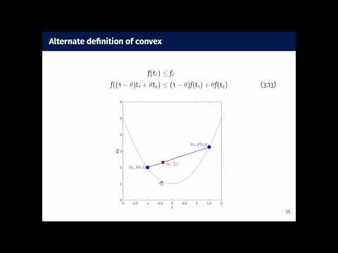
For points at t₁ and t₂, the segment between them is parameterized by (1−θ)p₁ + θp₂, with 0 ≤ θ ≤ 1.
A convex function lies on or below the chord joining (t₁, f(t₁)) and (t₂, f(t₂)); a concave function lies on or above it.
Strict convexity requires the graph to lie strictly below the chord at interior points; ordinary convexity permits equality.

13:30 Tangent-Line Inequality and Its Taylor Proof

For a differentiable convex function, every tangent line lies below the graph; the tangent at t₀ is f(t₀) + f′(t₀)(t−t₀).
Burton Ma derives the inequality using a second-order Taylor expansion: convexity makes the second-derivative remainder nonnegative.
The chord and tangent inequalities are standard tools in proofs about convex optimization, even though students are not expected to memorize their formal definitions for this course.

19:00 Why Multidimensional Optimization Uses Line Searches

Many multidimensional optimization algorithms reduce each iteration to a one-dimensional minimization along a chosen direction.
Line-search methods repeatedly solve these simpler 1D problems; quadratic approximation is one approach introduced earlier.
A line search still must handle multiple minima or the possibility that no minimum exists.

21:00 Finding a Minimum-Containing Bracket with Expanding Steps

A bracket uses t₁ < t₂ < t₃ with f(t₁) > f(t₂) and f(t₂) < f(t₃), giving evidence of a minimum inside the interval.
Starting from a point, move downhill until function values rise; doubling step sizes can find an endpoint with fewer evaluations than constant small steps.
Expanding steps may create a wide bracket containing multiple local minima, while smaller steps can locate a tighter interval at the cost of more function evaluations.

27:00 Bracketing Algorithm Inputs and Direction Pitfalls

The algorithm takes a starting point, an initial step size, and a growth factor k > 1, then expands the step until the function value rises.
If the first trial value is higher than the starting value, the algorithm reverses the step direction; it swaps endpoints afterward if needed so t₁ < t₃.
A large initial step can jump over a nearby minimum and falsely suggest the direction is wrong; derivatives can indicate downhill direction but may be unavailable or expensive to evaluate.

32:00 Dichotomous Search: Shrinking the Bracket Efficiently

A single midpoint evaluation cannot identify which half contains the minimum, so dichotomous search evaluates two interior points and retains a sub-bracket.
With probes at one-third and two-thirds of the interval, the bracket shrinks by a factor of 2/3 per iteration; reaching 1% of the initial width takes about 12 iterations.
Placing two distinct probes very close together can reduce the bracket by approximately one-half per iteration, reaching 1% in about 7 iterations—roughly 14 function evaluations versus 24.
The interval-reduction conclusions rely on strict convexity; after each comparison, the retained bracket is searched again until its width is sufficiently small.

Summary, takeaways, and chapters were generated by AI from the video's transcript and may contain errors. The video belongs to its creator, Burton Ma.