Lecture 3: Optimization via quadratic approximation (cont); Stationarity
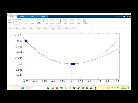 Watch on YouTube →
Overview
Burton Ma finishes the MATLAB implementation of quadratic interpolation for one-dimensional minimization, showing how function handles, bracket updates, iteration limits, and the backslash operator support the algorithm. He then develops stationarity conditions: a local minimum requires a zero first derivative and a nonnegative second derivative, but stationary points can also be maxima or inflection points.
Key takeaways
- Quadratic interpolation estimates a one-dimensional minimizer from three sampled objective values and updates a bracket so the minimum remains enclosed.
- MATLAB's @function syntax passes an objective through a function handle, while the backslash operator solves the parabola-coefficient system without explicitly forming a matrix inverse.
- A local minimum of a differentiable function must have zero first derivative, but zero derivative alone cannot distinguish a minimum from a maximum or a stationary inflection.
- For a twice-differentiable one-dimensional objective, a local minimum requires a nonnegative second derivative; positive curvature indicates convexity near the point.
- A stationary inflection combines zero first derivative with a sign change in the second derivative, so an algorithm that only targets stationary points may fail to find a minimum.
Chapters
0:00
Quadratic Interpolation Inputs, History, and MATLAB Function Handles
- The minimizer is bracketed by left and right points T1 and T3, with an interior point T2; a fitted parabola estimates the minimum.
- The MATLAB routine returns an estimated minimizer and minimum, plus histories of bracket locations and parabola parameters for plotting.
- MATLAB passes the objective function through a function handle, created with syntax such as @f and called like a function name.
- The routine stops when successive minimizer estimates differ by less than a tolerance or the iteration count reaches Imax.
8:00
Solving the Parabola Fit and Visualizing Bracket Updates
- Three function evaluations at T1, T2, and T3 form the right-hand side of a 3-by-3 Vandermonde system for the parabola coefficients.
- MATLAB's backslash operator solves the coefficient system more reliably in general than explicitly computing the matrix inverse.
- A plotting script uses the saved bracket and parabola history to display each iteration of the minimization.
- When the parabola's estimated minimum preserves the bracket condition, the algorithm shifts the relevant endpoint and repeats.
13:00
Interpolation Converges as the Parabola Fits the Objective Locally
- The plots show the bracket narrowing around the minimum as the routine repeatedly fits a parabola to three sampled points.
- Near the minimum, the parabola becomes a closer approximation to many well-behaved objective functions, improving the next estimate.
- The algorithm does not know the full plotted curve; it only evaluates the objective at discrete points.
- Convergence occurs when the change in the estimated minimizer falls below the chosen tolerance.
16:30
Why a Local Minimum Must Have Zero First Derivative
- Assuming a continuous, twice-differentiable objective, Burton Ma uses the difference quotient around a local minimizer to establish the first-order condition.
- To the right of the minimizer, the difference quotient is nonnegative; to the left, it is nonpositive.
- If the derivative is continuous and both one-sided limits agree, the derivative at the minimizer must equal zero.
- The zero-derivative condition is necessary but not sufficient: it identifies stationary points, not minima alone.
24:10
Stationary Minima, Maxima, and Inflection Points
- A stationary point is any location where the first derivative is zero, corresponding to a horizontal tangent.
- The illustrated function has three stationary points: one local minimum, one local maximum, and one point that is neither.
- A stationary point of inflection has zero first derivative but is not a local extremum; an optimization method that only seeks zero derivative can converge there.
- Concavity and convexity are characterized by the second derivative: negative indicates concavity, while positive indicates convexity.
28:10
Second-Order Minimum Condition and the Taylor Approximation
- At a local minimum, the second-order necessary condition is f''(t*) ≥ 0; a local maximum instead requires a nonpositive second derivative under the corresponding condition.
- The second-order Taylor expansion approximates a function locally by a quadratic using its value, first derivative, and second derivative at t*.
- At a minimizer, the first-derivative term vanishes, and the nonnegative change in function value supports the nonnegative-curvature condition.
- The classroom derivation is described as non-rigorous because it drops higher-order Taylor terms.
34:30
Inflection Points and the Terminology of Saddle Points
- An inflection point is where the second derivative changes sign, marking a transition between concave and convex behavior.
- A stationary point of inflection also has a zero first derivative.
- Some course notes call a one-dimensional stationary inflection a saddle point, but Burton Ma notes that technically saddle points apply to functions of more than one variable.
Summary, takeaways, and chapters were generated by AI from the video's transcript and may contain errors. The video belongs to its creator, Burton Ma.