Lecture 2: Optimization via quadratic approximation

Overview

Burton Ma introduces minimization concepts through a triangle-distance example, then develops a one-dimensional line search that fits a quadratic to three bracketed samples and repeatedly narrows the bracket. He explains local versus global minima, derives the parabola’s minimizer, and demonstrates MATLAB implementation details including stopping tolerances, iteration limits, Vandermonde systems, and solving with backslash rather than an explicit matrix inverse.

Key takeaways

A valid one-dimensional bracket requires t₁ < t₂ < t₃ and f(t₂) below both endpoint values, which confines a local minimum to the interval.
Quadratic interpolation estimates a local minimum from three function evaluations by solving a Vandermonde system and calculating t* = −a₂/(2a₁).
Updating the bracket according to the fitted minimum’s location and value progressively narrows the search, but cannot guarantee the global minimum.
The optimization algorithm sees function evaluations rather than the complete objective-function graph, so visual intuition from a plot is not available to the procedure itself.
In MATLAB, solve the coefficient system with A\y rather than inv(A)*y; the backslash solve is generally more numerically stable.
The demonstrated stopping rule checks the change in successive t* estimates against a default tolerance of 10⁻⁶ and also caps execution at 10 iterations.

Chapters

0:00 Triangle-Distance Minimization and MATLAB Contour Plots

The example minimizes the sum of distances from a point X to triangle vertices A, B, and C.
A MATLAB brute-force grid produces contour lines, each representing a constant objective value; one shown contour is about 5.99.
For one triangle, the approximate minimizer is (3.52, 1.56) with a distance sum near 4.83; changing the triangle can put the minimizer at a vertex.

5:00 Optimization Domains, Real Vectors, and Objective Functions

Optimization searches a set of candidates, such as a subset of the real numbers R or vectors in R² and Rⁿ.
The example sets include numbers between 0 and 1 and vectors with length less than 1, forming a unit disk in R².
An objective function maps a candidate to a real-valued cost; the triangle problem’s cost is the sum of its three vertex distances.

8:00 Minimizers, Minimum Values, and the Limits of Function Plots

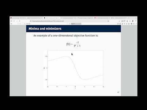
An optimization algorithm generally evaluates points rather than seeing the complete graph of the objective function.
The arg min identifies the input that minimizes a function, while min gives the function value at that input.
Maximization can be rewritten as minimization by negating the objective function.

14:00 Local and Global Minima on Restricted Domains

An exponentially damped sinusoid on the interval from 0 to 10 has eight local minima, but only one lowest value on that restricted domain.
A global minimizer has an objective value no greater than the value at any other point in the domain; a strict global minimizer is strictly lower.
Local minimizers are lowest within a neighborhood, and optimization algorithms can converge to one without finding the global minimum.

22:00 Bracketing a One-Dimensional Minimum

A bracket uses three ordered points t₁ < t₂ < t₃ with f(t₂) below both f(t₁) and f(t₃).
These inequalities establish that a minimum lies somewhere in the interval from t₁ to t₃, although multiple local minima may be present.
Line-search methods reduce higher-dimensional optimization tasks to a sequence of one-dimensional searches.

26:00 Fitting a Quadratic Through Three Bracket Samples

The method fits p(t) = a₁t² + a₂t + a₃ through the three evaluated points at t₁, t₂, and t₃.
The coefficients come from a 3×3 Vandermonde linear system whose rows use t², t, and 1.
A quadratic is useful because smooth functions often resemble a parabola near a local minimum, and its minimum is easy to calculate.

32:00 Calculating the Parabolic Minimum and Updating the Bracket

Setting p′(t) = 2a₁t + a₂ to zero gives the fitted parabola’s stationary point, t* = −a₂/(2a₁).
The bracket conditions determine which endpoint or interior point to replace, with four cases based on whether t* lies between t₁ and t₂ or t₂ and t₃ and how its fitted value compares with f(t₂).
Repeated bracket updates shrink the search interval; the method finds a local minimum within the bracket, not a guaranteed global minimum.

40:00 MATLAB Line-Search Function and Stopping Conditions

The MATLAB function q_fit_search accepts a function handle and three bracket points, with checks for real values and the ordering t₁ < t₂ < t₃.
The example uses a default tolerance of 10⁻⁶ and a maximum of 10 iterations; it stops when the estimated t* changes by less than the tolerance or the iteration limit is reached.
The implementation tracks function evaluations and can also store the history of t* estimates and fitted parabola coefficients.

44:00 Solving the Vandermonde System Stably in MATLAB

The fitted coefficients solve A a = y, where A is the Vandermonde matrix and y contains the three bracket-point function values.
MATLAB’s backslash operator, A\y, is preferred to explicitly computing inv(A)*y because it solves the system more numerically stably.
Vandermonde matrices can become poorly conditioned as powers grow, though the lecture’s fitting system is only 3×3.

Summary, takeaways, and chapters were generated by AI from the video's transcript and may contain errors. The video belongs to its creator, Burton Ma.