Lecture 10: Stationarity (multivariate)
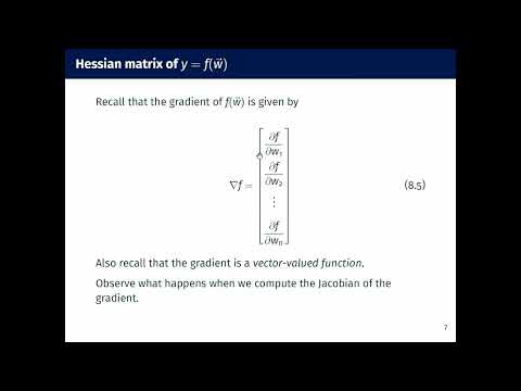 Watch on YouTube →
Overview
Burton Ma develops multivariate stationarity by connecting the gradient to first-order optimality and the Hessian to curvature through second-order Taylor approximations. He explains necessary and sufficient conditions using positive semidefinite and positive definite matrices, then applies Hessian tests to paraboloids and sums of sine functions to distinguish minima, maxima, and saddle points.
Key takeaways
- A multivariate stationary point requires ∇f(w*) = 0 because the directional derivative ∇f(w*)ᵀv must vanish for every direction v.
- At a local minimum, the Hessian must be positive semidefinite; a positive definite Hessian together with a zero gradient is sufficient for a strict local minimum.
- For a symmetric Hessian, eigenvalue signs classify a stationary point: all positive means a strict minimum, all negative a strict maximum, and mixed signs a saddle.
- The Hessian of (w₁² + w₂²)/2 is the identity matrix, so its eigenvalues are both 1 and its stationary point (0,0) is a strict minimum.
- For sin(w₁) + sin(w₂), stationary points occur where both cosine terms vanish, and the Hessian diag(−sin(w₁), −sin(w₂)) distinguishes minima, maxima, and saddles.
- A semidefinite Hessian alone can leave the classification unresolved, just as a zero second derivative does in one-variable calculus.
Chapters
0:00
Directional Derivatives Define Multivariate Stationarity
- A point w* is stationary when the directional derivative is zero in every unit-vector direction.
- Because the directional derivative equals the gradient dotted with direction v, vanishing for all v requires ∇f(w*) = 0.
- A zero gradient is necessary at a local minimum, but does not by itself distinguish minima from maxima or saddle points.
3:24
The Hessian Collects Second Partial Derivatives
- The Hessian is an n × n matrix of second-order partial derivatives, denoted H or ∇²f.
- For real-valued functions with continuous second partial derivatives, mixed partials agree, making the Hessian symmetric.
- The Hessian is related to the Jacobian of the gradient by transposition; when the Hessian is symmetric, they coincide.
8:27
Multivariate Taylor Series and the Hessian Quadratic Form
- The first-order approximation at w₀ is f(w₀) + ∇f(w₀)ᵀ(w − w₀), the tangent-plane analogue of a tangent line.
- The second-order approximation adds ½(w − w₀)ᵀH(w₀)(w − w₀), a quadratic form that captures local curvature.
- The gradient and Hessian replace the first and second derivatives used in the univariate Taylor expansion.
11:16
First- and Second-Order Conditions for a Local Minimum
- If w* is a local minimum, the first-order necessary condition is ∇f(w*) = 0.
- The second-order necessary condition is that H(w*) be positive semidefinite.
- If ∇f(w*) = 0 and H(w*) is positive definite, the second-order sufficient condition guarantees a strict local minimum.
17:15
Taylor-Based Proofs and Eigenvalue Bounds
- For the first-order argument, compare nearby points w* + hy and w* − hy; both must have function values at least f(w*), forcing the linear gradient term to vanish.
- In the second-order argument, the quadratic term yᵀH(w*)y must be nonnegative in every direction, which yields positive semidefiniteness.
- For a positive definite Hessian, the smallest eigenvalue λmin is positive and uᵀHu ≥ λmin for every unit vector u, giving a strictly positive local quadratic increase.
- The lecture presents these Taylor arguments as non-rigorous sketches because they omit control of higher-order remainder terms.
27:10
Matrix Definiteness and What It Says About Extrema
- For a real symmetric matrix M, positive definiteness means xᵀMx > 0 for every nonzero x; equivalently, all eigenvalues are positive.
- Positive semidefiniteness replaces the strict inequality with xᵀMx ≥ 0 and permits zero eigenvalues; indefinite matrices have both positive and negative eigenvalues.
- At a stationary point, a positive definite Hessian implies a strict local minimum, a negative definite Hessian a strict local maximum, and an indefinite Hessian a saddle point.
- A zero or merely semidefinite Hessian can be inconclusive, so additional analysis may be needed.
32:25
Paraboloid and Sine-Sum Examples in Two Dimensions
- For f(w₁,w₂) = (w₁² + w₂²)/2, the gradient is (w₁,w₂) and the Hessian is the identity matrix with eigenvalues 1 and 1.
- The paraboloid’s gradient vanishes at (0,0); its positive definite Hessian identifies that point as a strict local minimum.
- The surface f(w₁,w₂) = sin(w₁) + sin(w₂) has multiple minima, maxima, and saddle points, illustrated by viewing the surface from different directions.
- The examples are restricted to ℝ² because functions with three or more inputs are difficult to visualize directly.
39:00
Classifying Sine-Sum Extrema and an Inverted Paraboloid
- For sin(w₁) + sin(w₂), the gradient is (cos(w₁), cos(w₂)) and the diagonal Hessian is diag(−sin(w₁), −sin(w₂)).
- Stationary coordinates occur where each cosine is zero; the signs of the Hessian’s diagonal entries identify local minima or maxima, while mixed signs indicate saddles.
- Negating the paraboloid gives Hessian −I, which is negative definite everywhere; its stationary point at (0,0) is therefore a strict local maximum.
Summary, takeaways, and chapters were generated by AI from the video's transcript and may contain errors. The video belongs to its creator, Burton Ma.