Lecture 10 7

Overview

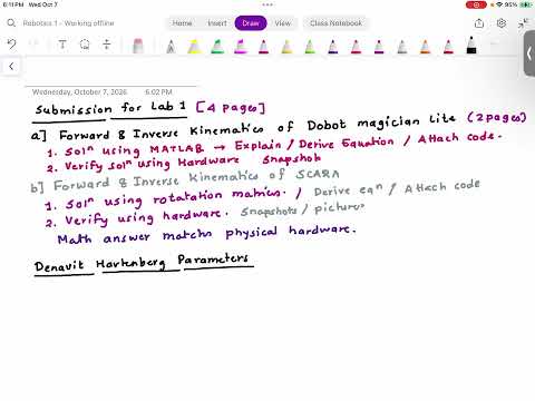
The lecture explains how to build Denavit–Hartenberg (DH) tables and use their homogeneous-transformation matrix to solve robot forward kinematics, while comparing the method with rotation matrices. It also sets Lab 1 requirements: MATLAB derivations and hardware verification for a Dobot and a SCARA robot, with a report of no more than four pages and snapshots showing measured joint angles and end-effector positions.

Key takeaways

A DH table has four parameters per frame transition—θ, α, r, and d—and its row count is the number of assigned frames minus one.
For the DH convention taught here, θ rotates about zₙ₋₁ to align the x axes, while α rotates about xₙ to align the z axes; confusing α’s rotation axis with the vector being rotated is a common mistake.
The worked perpendicular 2R example produces θ₁ and θ₂ as the joint variables, α₁ = +90°, α₂ = 0, r₁ = 0, r₂ = A2, d₁ = A1, and d₂ = 0.
DH transformations should match rotation-matrix transformations when the frame assignment, offsets, and rotation signs are consistent; the lecture recommends solving examples by both methods to check work.
Lab 1 requires hardware evidence as well as mathematics: Dobot and SCARA results should be checked against robot snapshots, including joint angles and end-effector coordinates, within a report capped at four pages.

Chapters

0:00 Lab 1 Part One: Dobot Kinematics and Hardware Verification

The first part covers forward and inverse kinematics for the Dobot, with a MATLAB solution and derived equations.
Verify the calculations on the physical robot and include snapshots showing joint angles and end-effector coordinates px, py, and pz.
Attach the MATLAB code and explain how the mathematical results match the hardware.

2:38 Lab 1 Part Two: SCARA Kinematics and Four-Page Report

The second part covers forward and inverse kinematics for a SCARA robot, deriving the solution by hand with rotation matrices.
Substitute joint parameters to calculate px, py, and pz, then compare those values with the physical robot using photos or screenshots.
Keep the report to a maximum of four pages; its conclusion should state whether the equations agree with the hardware.

5:38 Why Robotics Textbooks Teach the Denavit–Hartenberg Method

Denavit–Hartenberg parameters, commonly shortened to DH parameters, are presented as the standard approach in robotics textbooks.
The method maps a robot’s frame geometry to a DH table and then to homogeneous transformations.
The lecture contrasts this procedure with the previously taught rotation-matrix approach.

9:54 DH’s Serial-Manipulator Scope and the Rotation-Matrix Alternative

DH parameters are described as a black-box or “plug-and-chug” method: assign four values per joint and substitute them into a fixed matrix.
The lecture says DH is intended for serial manipulators, such as robot arms, rather than UAVs, UGVs, soft robots, or parallel systems.
Rotation matrices are recommended for broader robot geometries, and students are asked to solve problems both ways and compare results.

13:16 DH Setup: Draw the Kinematic Diagram and Assign Frames

Begin by drawing the kinematic diagram, marking revolute-joint rotation axes and prismatic-joint extension axes.
Represent link offsets with perpendicular distances even when the physical robot geometry looks different.
Assign a fixed frame 0, frames along the joints, and a final frame at the end effector; use right-handed coordinate systems.

16:00 The Four DH Columns and the Number of Table Rows

Each DH table has four columns: θ, α, r, and d; θ and α are angles, while r and d are distances.
The row count equals the number of frames minus one: two frames require one row, while four frames require three.
Finding the correct four parameters for every frame transition is identified as the central work of the method.

20:58 Substitute DH Parameters into the Homogeneous-Transformation Matrix

For each transition from frame n−1 to frame n, substitute θₙ, αₙ, rₙ, and dₙ into a fixed 4×4 homogeneous-transformation matrix.
For example, calculate ⁰H₁ using the first table row and ¹H₂ using the second row.
The matrix provides the transformation without separately constructing rotation and projection matrices for each step.

27:07 How to Determine θ: Rotate About the Previous Frame’s Z Axis

θₙ is the rotation about zₙ₋₁ that aligns xₙ₋₁ with xₙ.
Add any fixed angular offset between the x axes to the revolute-joint variable; if the axes already align, the fixed offset is zero.
The lecture illustrates a positive 90-degree offset when rotating xₙ₋₁ into alignment with xₙ.

35:58 How to Determine α: Rotate About the New Frame’s X Axis

αₙ is measured about xₙ to align zₙ₋₁ with zₙ, making the axis used for rotation different from the vector being rotated.
To reason about the angle, redraw zₙ₋₁ in the new frame and measure its positive rotation to zₙ.
The lecture identifies α as a frequent source of errors and distinguishes it from the joint variable, which appears in θ.

45:30 How to Determine r: Measure the Offset Along the New X Axis

rₙ measures the displacement from the origin of frame n−1 to frame n along xₙ.
An offset of length a in the positive xₙ direction gives rₙ = +a when moving from the earlier frame to the later one.
If frame origins differ in both xₙ and yₙ, only the xₙ component contributes to r; the lecture labels that component B and excludes C.

51:21 How to Determine d: Measure the Offset Along the Joint-Axis Direction

Determine dₙ by measuring the displacement between frame origins along the relevant z-axis.
The lecture emphasizes tracking the direction from frame n−1 to frame n to assign a positive or negative sign.
Once θ, α, r, and d are identified for every row, substitute each row into the transformation matrix.

55:43 Set Up a Two-Link Perpendicular Revolute Robot for Comparison

The worked example is a two-degree-of-freedom robot with two revolute joints arranged perpendicular to one another.
The link lengths are labeled A1 and A2, and the requested transformations are ⁰H₁ and ¹H₂.
Students are first asked to solve the same geometry using rotation matrices before comparing it with the DH result.

59:29 Assign DH Frames and Build a Two-Row Table for the 2R Example

The robot has two joints and three frames, so its DH table contains two rows and the columns θ, α, r, and d.
The first joint axis is vertical and the second is horizontal; x₁ is selected to intersect z₀ while remaining perpendicular to it.
The third frame is placed at the end effector, completing the frame sequence used for ⁰H₁ and ¹H₂.

1:03:40 Worked Example: Identify θ₁ and θ₂ for the Perpendicular 2R Robot

For the first row, x₀ and x₁ are aligned, so θ₁ has zero fixed offset and equals the first revolute-joint variable.
For the second row, x₁ and x₂ are aligned, so θ₂ likewise equals the second revolute-joint variable.
The table’s θ column is therefore populated by the two joint variables, θ₁ and θ₂.

1:08:54 Worked Example: Find α₁ and α₂ from the Joint-Axis Directions

For α₁, rotate about x₁ to align z₀ with z₁; the example assigns a positive 90-degree twist.
For α₂, z₁ and z₂ are already aligned, so the second twist is zero.
The example highlights that α’s rotation is about the new x axis while the previous z axis is the vector being aligned.

1:12:48 Worked Example: Assign r and d from Link Lengths A1 and A2

The first frame-origin offset lies along z₀ rather than x₁, giving r₁ = 0 and d₁ = A1.
The second link length A2 lies along x₂, giving r₂ = A2.
There is no second-row displacement along the joint-axis direction, so d₂ = 0.

1:22:20 Calculate ⁰H₁ and Check It Against the Rotation-Matrix Result

Substitute θ₁, α₁ = 90°, r₁ = 0, and d₁ = A1 into the DH matrix to obtain ⁰H₁.
The resulting 4×4 matrix contains the rotation in its upper-left 3×3 block and translation components in its final column.
The lecture checks that this transformation matches the result previously derived using rotation matrices.

1:28:20 Calculate ¹H₂ and Compare Both Kinematics Methods

For the second row, substitute θ₂, α₂ = 0, r₂ = A2, and d₂ = 0 into the same DH matrix.
The resulting ¹H₂ is compared with the earlier rotation-matrix transformation for the second link.
The worked example’s conclusion is that DH parameters and rotation matrices yield the same transformations when the frames and signs are chosen consistently.

1:33:11 Quiz: Fill a DH Table and Verify ⁰H₁ and ¹H₂

The quiz revisits an earlier two-revolute-joint problem with joint variables θ₁ and θ₂ and link distances A1, A2, A3, and A4.
Students must construct the DH table, identify each θ, α, r, and d, and derive ⁰H₁ and ¹H₂.
Compare the DH results with the rotation-matrix answers already in the notes, then photograph the work and upload it to Canvas.

Summary, takeaways, and chapters were generated by AI from the video's transcript and may contain errors. The video belongs to its creator, ssredkar.