IEE 475: Lecture F (2026-10-01): Midterm Review

Overview

Ted Pavlic reviews IEE 475’s midterm topics, from discrete-event simulation terminology and Arena’s inverse-CDF functions to random-number generation, probability distributions, and goodness-of-fit tests. He also explains the two-stage Canvas exam: Stage 1 is a timed, lockdown-browser assessment worth 80% of the midterm score, and Stage 2 is an open-book collaborative assessment worth 20%.

Key takeaways

Arena’s DISC function encodes a discrete inverse CDF as alternating cumulative probabilities and outcomes; cumulative probabilities must be nondecreasing and end at 1.0.
The midterm combines a timed Stage 1 worth 80% with an open-book collaborative Stage 2 worth 20%; both stages contain the same questions, and only the latest Stage 2 submission is graded.
When integrating a piecewise PDF, interval limits supply constants needed for a continuous, nondecreasing CDF that starts at 0 and ends at 1.
An inverse-transform generator must map the full uniform interval [0,1] into the random variable’s support; checking compositions of the CDF and inverse can expose incorrect algebra or branch choices.
Uniformity and independence are the two required PRNG properties, and a uniformity test that rejects its null hypothesis has detected nonuniform values.
For chi-square uniformity tests, the expected count under the null—not the observed count—in each bin must be at least five; KS degrees of freedom use n, while chi-square uses bins minus one.

Chapters

0:00 Arena DISC Syntax for Discrete Inverse-Transform Sampling

The discrete inverse-transform method selects outcome xᵢ when a uniform random number falls between the relevant CDF bounds.
Arena’s DISC function takes alternating arguments: cumulative-probability values first, then their corresponding outcomes.
CDF arguments must be nondecreasing and the final cumulative probability must be 1.0.
DISC represents discrete stair steps; Arena’s CONT function connects empirical CDF points with ramps, interpolating between observed values.

7:01 Midterm Stages, Timers, and Canvas Availability

Stage 1 is available Monday through Wednesday in LockDown Browser with Monitor; its 90-minute timer accommodates technical issues, though the exam is designed for a 75-minute class period.
Stage 2 is available Thursday and Friday, open-book and open-notes, and permits collaboration with classmates.
The two stages use the same questions; students may record Stage 1 answers to use during Stage 2.
Stage 1 counts for 80% and Stage 2 for 20% of the midterm score; Stage 2 permits multiple submissions, but only the latest is graded.

13:19 Unlocking Midterm Materials and Study Resources

Complete the brief LockDown Browser compliance test in Unit F1 to unlock the midterm module in Unit F2.
The module includes eight sample midterms, including Fall 2025, with practice versions and solution sets.
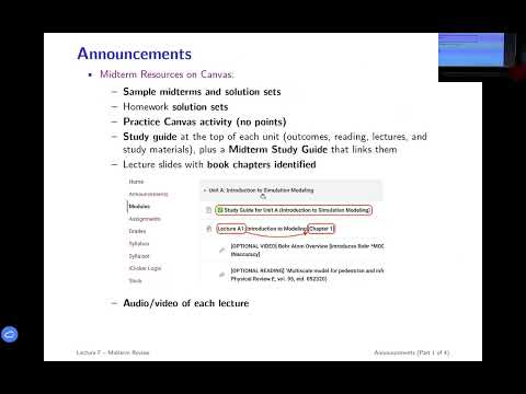
Homework solutions, repeatable Canvas practice activities, lecture recordings, textbook chapter references, and unit study guides are available.
Study guides list learning objectives; checking off those skills is intended to indicate readiness for each unit.

16:43 Allowed Aids and Expected Midterm Question Formats

Students may use a two-sided handwritten formula sheet, Canvas’s on-screen calculator, and a physical calculator.
Expect mostly autograded conceptual items—multiple choice, select-all, matching, and numerical fill-ins—with one or two design problems.
Possible quantitative tasks include inverting a CDF, generating LCG values, completing a hand-simulation table, or calculating a uniformity-test statistic.
All questions carry equal point value; statistical tables will be supplied, but the runs-above-and-below-the-mean test formulas will not.

24:16 Discrete-Event Simulation Vocabulary and Event Calendars

Review the distinctions among events, activities, delays, state variables, states, entities, attributes, and resources.
An event calendar lets discrete-event simulation jump directly to the next scheduled event instead of advancing through every time increment.
In an M/M/1 queue with continuing arrivals, schedule only the next arrival; the next interarrival time is not known until another random value is drawn.
Starting service schedules a future departure event; Arena’s Step control and event calendar can help inspect a simulation event by event.

26:44 LCG Indexing, KS Details, and Uniformity-Test Interpretation

For a linear congruential generator, the seed x₀ produces x₁, and the first uniform value is r₁ = x₁ divided by the modulus; x₀ is not itself the first random number.
Keep place value straight when converting an integer state into a value between 0 and 1, and compare decimal values carefully when selecting a maximum.
For the KS test, degrees of freedom are the sample count n; for chi-square, degrees of freedom are the number of bins minus one.
Uniformity-test null hypotheses assert that values are uniform; rejecting the null indicates nonuniformity, not a general verdict about every kind of randomness.

32:31 Integrating Piecewise PDFs into Continuous CDFs

Integrate each piece of a piecewise PDF using its correct interval limits; taking antiderivatives row by row without constants can create jumps and a function that is not a valid CDF.
A valid continuous CDF starts at 0, ends at 1, and is nondecreasing; continuity across interval boundaries checks that accumulated constants are correct.
Each later CDF interval includes probability accumulated over the earlier PDF pieces plus the contribution from the current interval.
For the reviewed example, the density changes across boundaries at 0.5, 1.5, and 2, so those limits determine the integration constants.

37:17 Choosing Inverse-CDF Intervals and Checking the Result

The random variable’s support is where its CDF increases; in the example, the support runs from 0.5 to 2, while constant CDF regions lie outside it.
Invert each nonconstant CDF segment separately and determine its corresponding R interval by evaluating the segment at its x-boundaries.
The resulting inverse-transform generator must map all of [0,1] into the support of the random variable.
Check the work by composing the CDF and inverse: applying one after the other should recover the original x or r value.

41:38 Selecting the Correct Branch When Inverting a Quadratic CDF

A CDF based on (x + 1)² uses only the increasing branch from x = −1 to x = 0, even though the full quadratic is not one-to-one.
Solving for x creates positive and negative square-root branches; choose the branch whose outputs remain within the support [−1, 0].
For uniform r in [0,1], the wrong branch produces values below −1, so it cannot generate the stated random variable.
CDFs are graphically invertible on their increasing portions, so inversion must preserve the specific portion used by the CDF.

45:12 Models as What-If Tools and Simulation Model Types

Pavlic defines a model as anything that helps answer a “what if” question; it need not be mathematical or computational.
Models act like microscopes: they isolate a possible cause or slice of reality to test for insight rather than copying the entire real system.
Stochastic models use randomness; agent-based models can represent spatial effects but require more parameters, while system-dynamics models are deterministic and suited to long-range behavior.
Discrete-event simulation terminology—especially entities, attributes, resources, activities, and delays—is foundational exam material.

49:41 Activities, Delays, and Hand-Simulating Queue Events

Activities are modeled inputs known probabilistically in advance, such as service time or an interarrival time; delays are outcomes that depend on the system’s evolving state.
Airport document-check duration is an activity, while time spent waiting to reach an agent is a delay affected by the queue.
Hand-simulation questions may blank out event times or departure counts, and could vary from an M/M/1 queue to a capacity-two M/M/2-style server.
A queue’s future-event list should contain only events that are currently known, not arrivals inferred from future random values.

53:58 Distribution Families, Input Models, and the Poisson Process

Know the rough ranges, parameters, shapes, and typical uses of the six continuous and five discrete distributions listed in the course review slides.
PMFs describe discrete probabilities, PDFs describe continuous density, and CDFs accumulate probability; skewed shapes are inconsistent with a normal distribution’s symmetry.
A homogeneous Poisson process has exponentially distributed interarrival times and Poisson-distributed counts in an interval.
For a Poisson process with rate λ over interval length t, the count’s mean is λt; Pavlic says nonhomogeneous-process details are not a midterm focus.

59:55 PRNG Requirements, LCGs, and Combined Generators

The required properties of a pseudorandom number generator are uniformity and independence; speed, long period, and reproducibility from a seed are desirable features.
Changing seeds helps produce independent simulation replications, even though seed-based repeatability is not one of the two basic PRNG requirements.
Know the linear congruential generator formula and how to generate values or infer a missing parameter such as the multiplier.
LCGs have limited periods; combining generators can produce much longer cycles.

1:04:21 Chi-Square, KS, and Runs-Above-and-Below-Mean Tests

For a chi-square uniformity test, expected observations per bin under the null must be at least five; use equal-width bins over [0,1], not just the observed sample range.
Compute the chi-square statistic by summing (observed − expected)² / expected across bins, then compare it with the supplied table using bins minus one degrees of freedom.
The KS test suits smaller samples: sort the values, compare empirical and uniform CDF values, take the largest discrepancy, and use n as its degrees of freedom.
The runs test converts observations above and below the mean to a binary sequence, counts runs, and uses formulas for the null mean and variance; for a two-tailed 5% test, compare the z statistic with 1.96.

Summary, takeaways, and chapters were generated by AI from the video's transcript and may contain errors. The video belongs to its creator, Ted Pavlic.