IEE 475: Lecture E2 (2026-09-29): Random-Variate Generation

Overview

IEE 475 Lecture E2 covers how to test pseudo-random number generators for uniformity and independence, then convert uniform draws into distribution-specific samples using inverse transforms. It works through chi-square and Kolmogorov–Smirnov tests, a runs-above-and-below-the-mean test, Arena seed streams, and inverse CDF derivations for exponential and triangular distributions.

Key takeaways

A chi-square uniformity test uses equal-width bins defined by the hypothesized interval, not by the observed minimum and maximum; with 30 observations and four bins, each expected count is 7.5.
Chi-square testing requires expected counts of at least 5 per bin; for small samples, the KS test instead measures the maximum gap between the sample CDF and the hypothesized CDF.
A KS test’s failure to reject does not prove uniformity, but its high power makes it useful for detecting departures with small samples; large samples can make it overly sensitive to minor deviations.
The runs-above-and-below-the-mean test converts numeric draws into a binary sequence and tests its run count; the example’s 19 runs produce z = 1.23, below the two-sided 5% threshold of 1.96.
Arena’s named random streams and editable seeds make simulation replications reproducible and let modelers control which random sequence drives arrivals, service, or other processes.
Inverse-transform sampling derives an output from a uniform draw by solving R = F(x); the exponential sampler is −ln(1 − R)/λ, while triangular sampling requires separate inverse branches.

Chapters

0:00 Homework D2: Histogram the Generated Variates

Homework D2 is due Saturday, with solutions planned for Sunday before the midterm opens.
Histogram the generated random variates, not the uniform input random numbers; a flat histogram can indicate the wrong Excel column was selected.
Submit a DOCX or PDF report with results and histograms, rather than a spreadsheet of raw numbers.
Organize responses in question order and write concisely for the TA who must grade roughly 60 submissions.

3:00 Midterm Format, Schedule, and Practice Resources

The midterm’s individual Stage 1 is closed-book and closed-notes, uses LockDown Browser with a camera, and allows two formula sheets.
Stage 1 has a 90-minute timer, though the exam is designed for 75 minutes; Stage 2 opens Thursday, is collaborative and open-resource, and contributes 20% of the score versus 80% for Stage 1.
The exam availability is at least Monday and Tuesday, with Wednesday still under consideration; the lockdown-browser compliance test unlocks the midterm module.
The module includes about eight practice exams dating back to Fall 2025, along with additional review materials.

7:55 Distribution Vocabulary and the Inverse-Transform Idea

The core distribution families include uniform, triangular, normal, exponential, Erlang, Weibull, beta, Bernoulli, binomial, negative binomial, and geometric.
For each distribution, know its use cases, support, number of parameters, and how the parameters affect its shape.
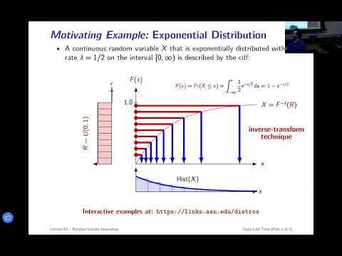
Inverse-transform sampling starts with a PDF, integrates it to obtain a CDF, and sets the CDF equal to a uniform draw R to solve for X.
The transformation stretches uniform inputs into outputs whose distribution matches the target PDF.

11:00 PRNG Seeds and Named Streams in Arena

A random number means a uniform draw on [0,1]; a random variate follows a specified distribution, and a PRNG produces reproducible pseudo-random sequences.
Excel RAND does not expose a user-controlled seed, whereas simulation tools need repeatable seeds to revisit interesting replications.
Arena’s Seeds element lets users edit the default stream, identified as stream 10, or create named streams such as arrival and service streams.
Arena can advance or initialize seeds across replications; expressions can accept a stream ID to control which random stream a process uses.

16:47 The Two Required PRNG Properties: Uniformity and Independence

Uniformity requires draws to be spread across the full 0-to-1 interval rather than clustered in a few regions.
Independence means earlier draws should not predict later draws; an ordered sequence can be uniform yet still violate independence.
The class uses chi-square and Kolmogorov–Smirnov tests for uniformity, and a runs test for independence.
Seed control supports reproducible, independent simulation replications and later variance-reduction experiments.

22:33 Chi-Square Uniformity Test with Four Equal-Width Bins

For a uniformity test on [0,1], four bins must be equal-width: [0, 0.25), [0.25, 0.5), [0.5, 0.75), and [0.75, 1].
With 30 observations, observed bin counts of 3, 4, 8, and 15 compare against an expected count of 7.5 per bin.
Compute the statistic as the sum of (observed − expected)² / expected; do not square the expected count in the denominator.
Four bins give 3 degrees of freedom; at a 5% significance level the critical value is 7.81, so a larger statistic rejects uniformity.

31:39 Kolmogorov–Smirnov Test for Small Samples

Use the KS test when sample sizes are too small for chi-square’s expected-count requirement of at least 5 per bin.
Sort the observations and compare their sample CDF, represented by rank-based steps, with the uniform CDF’s diagonal line.
For five sample values, the test statistic is the largest CDF deviation; the worked example gives D = 0.26 against a 5% critical value of 0.56.
Failing to reject uniformity does not prove it, but a small-sample KS test has high power and can provide useful evidence.

39:53 Interpreting Test Results and Moving Independence Checks to Software

Software in MATLAB, R, and Python can run chi-square and KS tests and return p-values instead of requiring manual table lookups.
Compare a p-value with alpha: reject the null hypothesis when p < alpha, and otherwise fail to reject it.
The independence tests target autocorrelation—whether earlier sequence values help predict later ones—and belong to the runs-test family.
A lattice or return-map scatter plot can also reveal structure in poor PRNGs, but the course focuses on the runs-above-and-below-the-mean test.

45:36 Runs Above and Below the Mean: Convert Draws into a Binary Sequence

Use the supplied mean to map each observation to 0 if it is below the mean and 1 if it is above it.
For the 30-observation example, the sequence contains 13 zeros and 17 ones.
A run is a contiguous group of identical outcomes; count a new run each time the sequence switches between 0 and 1.
The example has 19 runs, including single-element runs when a value is immediately followed by the other category.

53:57 Runs-Test Z Score and Combined Linear Congruential Generators

Under independence, the example’s run count has expected value 15.7 and variance 6.9; standardize 19 using the square root of the variance to get z = 1.23.
For a two-sided 5% test, compare |z| with 1.96; since 1.23 is smaller, the example does not reject independence.
A basic linear congruential generator can have acceptable uniformity and independence yet still repeat after a relatively short period.
A combined LCG combines sequences with different periods to produce a much longer cycle, rather than serving primarily as a uniformity test.

56:43 Arena Distribution Expressions and Inverse-Transform Sampling

Arena delay expressions can specify distributions such as a uniform draw between 2 and 4, and optional stream IDs select a particular random-number stream.
The general inverse-transform procedure is to integrate the PDF, set R equal to the CDF, and solve for X as a function of R.
When a CDF cannot be inverted in closed form, other sampling methods exist, though they are outside the main derivations here.
The resulting expression maps uniform PRNG draws to samples from the desired distribution.

58:18 Exponential Variates from the Inverse CDF

For an exponential distribution with rate parameter λ, integrating its piecewise PDF gives CDF F(x) = 0 for x < 0 and 1 − e^(−λx) for x ≥ 0.
Set R = F(x) and solve to obtain the inverse sampler x = −ln(1 − R) / λ.
Because 1 − R is also uniform when R is uniform, implementations often use −ln(R) / λ to avoid an extra subtraction.
The formal exam derivation uses the 1 − R form before that implementation optimization.

1:02:23 Deriving the Triangular Distribution CDF

A triangular distribution’s piecewise PDF produces a piecewise CDF across the lower bound a, mode c, and upper bound b.
When integrating each region, carry the accumulated probability from the previous region so the CDF remains continuous at a and c.
Check that the CDF starts at 0, ends at 1, is nondecreasing, and has no jumps for a continuous triangular variate.
The mode c marks the change between the rising and falling portions of the density.

1:05:40 Invert the Triangular CDF and Select Valid Square-Root Branches

Split the inverse sampler into two cases, using the CDF’s probability ranges corresponding to a-to-c and c-to-b.
Set R equal to the relevant CDF segment and solve each equation for X; flat CDF regions do not need inversion.
Choose the square-root signs so samples remain within [a,b]: the lower branch rises from a, while the upper branch approaches b.
The lecture closes with a clicker prompt instructing students to choose option C.

Summary, takeaways, and chapters were generated by AI from the video's transcript and may contain errors. The video belongs to its creator, Ted Pavlic.