IEE 475: Lecture D2 (2026-09-22): Probabilistic Models
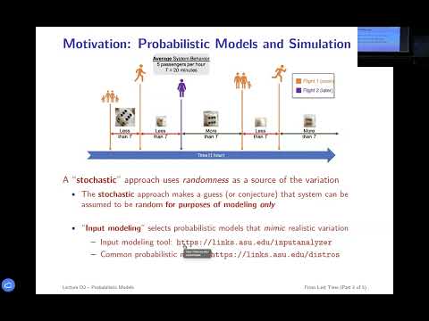 Watch on YouTube →
Overview
Ted Pavlic builds the probability vocabulary used to create input models for discrete-event simulations, distinguishing PMFs, PDFs, CDFs, expected values, and measures of spread. He then gives practical selection rules for common distributions: use uniform or triangular models for bounded values, normal models when mean and spread are known, and exponential models for nonnegative durations with a known mean or constant hazard rate; Erlang, Weibull, and Poisson models extend these ideas.
Key takeaways
- A PDF’s height is not a probability: a uniform density of 2 on [0, 0.5] is valid because its area is 1.
- CDFs provide one framework for both discrete and continuous variables: they are nondecreasing, range from 0 to 1, and give interval probabilities by subtraction.
- When only bounds are known, use a uniform model; when bounds and a most-likely value are known, use a triangular model.
- When an unbounded variable is specified by its mean and standard deviation, a normal distribution is the maximum-entropy choice; sums of independent stages also tend toward normality.
- For a nonnegative duration with a known mean and no known upper bound, an exponential model is appropriate when a constant hazard rate or memoryless behavior is plausible.
- Poisson counts and exponential interarrival times describe connected views of an arrival process: one counts events per period, while the other models the time between them.
Chapters
0:00
Arena Labs, Software Access, and Textbook Version Differences
- Labs 5–10 use Arena; later lab sessions are reserved for final-project work.
- Arena is available on campus lab computers, through Windows installations such as Parallels or VMware, and through Canvas’s Aporto virtual desktop.
- Arena versions before 16.1 use an older interface; textbook screenshots may differ, but the old features remain in the newer ribbon interface.
4:00
Random-Number Homework, Submission Expectations, and Midterm Format
- In the C2 random-number assignment, each modulus remainder becomes the next seed; the next iteration must use the value after the modulus.
- Homework submissions should consolidate work into one readable document; C2’s first five random-number calculations must show the hand-worked formula steps.
- The midterm has two stages: a proctored LockDown Browser exam on Tuesday and an open-notes, open-collaboration stage on Thursday.
12:00
Midterm Practice Resources and Arena Competition
- The Canvas midterm review can be attempted repeatedly, draws new randomized questions each time, and keeps the highest score.
- Completing the LockDown Browser compliance check unlocks the midterm module, which contains sample exams from the previous eight years.
- The optional Arena competition entry is due October 3; students should confirm Arena access before lab deadlines.
13:15
Stochastic Input Models and Random-Variable Ranges
- Discrete-event simulations represent variation with probability distributions, even when real-world events are deterministic but impractical to reproduce step by step.
- An input model is a probability distribution used as a surrogate for observed system behavior, such as interarrival times in a queue.
- A random variable maps real-world outcomes to numbers; its range determines whether it is discrete, with a countable set of values, or continuous.
16:30
PMFs, PDFs, and Why Density Can Exceed One
- A discrete random variable assigns probability mass to individual outcomes through a probability mass function (PMF); all outcome probabilities sum to one.
- A continuous variable uses a probability density function (PDF), whose area—not height—over an interval gives probability.
- PDF values may exceed one because density has units of probability per unit of x; for example, a uniform distribution on [0, 0.5] has density 2 and total area 1.
21:30
CDFs Unify Discrete and Continuous Probability Models
- The cumulative distribution function is F(x) = P(X ≤ x) for both discrete and continuous random variables.
- For a discrete variable, cumulative probabilities are added; for a continuous variable, density is integrated from negative infinity to x.
- A valid CDF is nondecreasing, begins at 0, and approaches 1; interval probabilities are calculated as F(upper) − F(lower).
27:00
Reading Discrete CDFs and Using the Inverse-Transform Method
- For service times of 3, 6, or 10 minutes with probabilities 0.30, 0.45, and 0.25, the CDF steps to 0.30, 0.75, and 1.00.
- A discrete CDF is defined between its outcome values as well as at them; for example, F(7) remains 0.75 in this service-time example.
- The inverse-transform method maps a uniform random number on [0, 1] through an inverse CDF to generate samples with the desired probabilities.
31:50
Continuous CDFs and Generating Exponential Random Values
- An exponential CDF rises quickly near zero and approaches 1 asymptotically, reflecting many short durations and fewer long ones.
- Inverting the exponential CDF converts uniform random draws from Excel, MATLAB, or R into exponentially distributed samples.
- CDF-based views avoid histogram bin-size choices and also provide a direct route to calculating probabilities and generating simulation inputs.
38:00
Expected Value, Variance, and the Center-of-Mass Analogy
- The mean or expected value is a distribution’s balance point; an average or sample mean is calculated from observed data.
- The center-of-mass analogy explains why the mean provides a useful single-point summary of a distribution, while still discarding its variation.
- Variance is the expected squared distance from the mean, and standard deviation is the square root of variance; higher moments also describe features such as skew.
51:00
Distinguishing PDFs, CDFs, and Inverse CDFs by Their Shapes
- A PDF must be nonnegative and have total area 1; it can rise above 1, so height alone cannot disqualify it.
- A CDF must stay between 0 and 1, be nondecreasing, and run from 0 to 1; negative x-values are allowed because x represents outcomes, not probabilities.
- An inverse CDF maps probabilities in [0, 1] to outcome values; a graph that assigns multiple outputs to one input is not a function and cannot be a PDF or CDF.
54:45
Uniform Distribution for Bounded Values with No Further Information
- If stakeholders provide only lower and upper bounds a and b, the uniform distribution is a low-bias default and the maximum-entropy choice under those constraints.
- Uniform outcomes do not favor any point within the interval [a, b].
- The probability of falling in a subinterval equals its length divided by the full range; an interval of length 2.5 within a range of 10 has probability 0.25.
57:10
Triangular Distribution for Bounds and a Most-Likely Value
- Use a triangular distribution when stakeholders provide a minimum a, maximum b, and most-likely value c.
- The density rises toward c on the left and falls away from c on the right, encoding the stated mode without adding an unsupported shape assumption.
- In the CDF, the inflection point marks the mode; multiple inflection points can signal a multimodal distribution.
1:00:35
Normal Distribution for Known Mean, Spread, and Additive Processes
- When an unbounded variable is described by its mean and standard deviation, the normal distribution is the maximum-entropy model given those values.
- The central limit theorem explains why sums of independent stages tend toward a normal shape; a sequence of roughly 20 or more stages is likely to be close to normal.
- A normal model can approximate positive quantities when the mean is many standard deviations above zero; a truncated normal is another option when negative values must be excluded.
1:06:35
Exponential, Erlang, Weibull, and Poisson Arrival Models
- For a nonnegative variable with a known mean but no stated upper bound, the exponential distribution is a practical default; it also models waiting time under a constant hazard rate.
- Exponential waiting times are memoryless: elapsed waiting time does not change the remaining-wait distribution, unlike scheduled bus arrivals that become more imminent over time.
- An Erlang-k variable is a sum of k exponential stages and approaches a normal shape as k increases; the Weibull adds a shape parameter for flexible reliability and failure-time models.
- Poisson distributions model discrete arrival counts over a period, while exponential distributions model the associated interarrival times; the next lecture introduces Bernoulli-based models.
Summary, takeaways, and chapters were generated by AI from the video's transcript and may contain errors. The video belongs to its creator, Ted Pavlic.