IEE 475: Lecture D1 (2026-09-17): Probability and Random Variables

Overview

Ted Pavlic builds the probability vocabulary needed for input modeling and simulation: random variables map outcomes to numbers, discrete variables use probability mass functions, continuous variables use density functions, and cumulative distribution functions unify both. He connects probability to physical mass and center of mass, explains inverse-CDF generation from uniform random numbers, and defines expectation, variance, and standard deviation; course logistics also cover Arena, assignments, and the two-stage midterm.

Key takeaways

Input modeling selects probability distributions for simulation inputs such as interarrival times and customer demand; simulated entities are separate from those distributions.
Discrete random variables have finite or countably infinite ranges and are described by PMFs whose outcome probabilities sum to 1; their plots should use isolated stems, not interpolating lines.
A continuous PDF represents probability per unit of the variable, not probability itself: it may exceed 1, while the area under it over an interval gives probability and any single point has zero probability.
For either discrete or continuous variables, a CDF gives the probability of being at or below a threshold; interval probability is the upper CDF value minus the lower one.
Inverse-CDF sampling converts uniform draws on [0,1] into samples from a target distribution, including geometric and exponential distributions that may lack built-in software generators.
The mean is the distribution’s center of mass, while variance is the second central moment and can be calculated as E[X²] − E[X]²; standard deviation is the square root of variance.

Chapters

0:00 Course Roadmap, Arena Access, and Upcoming Assignments

The next two and a half weeks move from probability and random variables to modeling distributions, random-number generation, random-variate generation, and midterm review.
Lab 5 introduces a basic queuing system in Arena; students can use campus lab machines, a Windows student installation, or the Apporto portal.
Homework C2 covers random-number generation; for its hand calculations, show each formula substitution rather than only submitting a table of results.
The modulo operation returns a remainder—for example, 5 mod 3 = 2—and helps bound generated numbers to a required range.

6:00 Midterm Review, Two-Stage Exam, and Software Logistics

Homework D2 covers random-variate generation and includes some calculus and algebra; its solutions are intended to be available before the midterm.
The midterm review assignment can be attempted repeatedly, with the highest score recorded; the review lecture includes questions and material from earlier lectures.
Stage 1 is a 90-minute, closed-book exam worth 80% of the midterm, with two student-produced double-sided reference sheets and video proctoring.
Stage 2 is worth 20%, is collaborative with classmates and open-book, and is unproctored; sample midterms are available online.

12:15 Stochastic Modeling and the Purpose of Input Distributions

Stochastic modeling represents real-world variation with probability distributions instead of replacing a process with only its average behavior.
For example, arrivals averaging one person every 20 minutes can still cluster, capturing operational variation that a fixed 20-minute interval would miss.
Input modeling selects distributions—such as interarrival times or customer product demand—to feed into a larger simulation; the inputs are not the simulated entities.
Pavlic distinguishes stochasticity, the use of randomness in modeling, from randomness as a general synonym.

15:30 Probability as Measure Theory: Mass, Density, and Balance

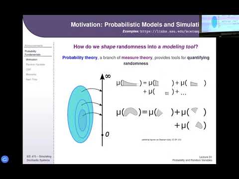
Probability belongs to measure theory, which studies measures that assign consistent quantities to sets and their parts.
A probability measure assigns total mass 1 to the full sample space and keeps the probabilities of mutually exclusive outcomes additive.
Pavlic uses physical mass as an analogy: uniform density gives equal mass to equal-length slices, while a distribution’s mean acts like its center of mass.
The terms probability mass and probability density reflect this physical analogy, which will recur when comparing discrete and continuous distributions.

19:20 Random Variables, Sample Spaces, and Ranges

A random variable is a function mapping outcomes from a sample space to a measurable space, often the real number line; despite its name, it is a mapping rather than a randomly changing variable.
For a coin flip, a random variable might map heads to 1 and tails to 0; choosing different numerical labels is a choice of mapping.
The sample space contains mutually exclusive outcomes, while the random variable’s range is the subset of real numbers those outcomes map to.
The support refers to values with nonzero probability or density, a concept used alongside range when describing distributions.

23:53 Events and the Probability Measure

An event is a set of outcomes, so events can overlap even though individual outcomes are mutually exclusive.
For a 20-sided die, the event “5 or less” overlaps with the event “even”; their probabilities therefore cannot simply be added as if the events were disjoint.
A probability measure assigns nonnegative weights to events, gives the full sample space weight 1, and defines an event’s weight as the sum of its outcome weights.
Probability questions typically ask about events, such as a die showing at least four dots, rather than only one isolated outcome.

27:28 Discrete Random Variables, PMFs, and Correct Plotting

A discrete random variable has a finite or countably infinite range; counts such as cars passing a point can take nonnegative integer values even when unbounded.
Its probability mass function assigns nonnegative probabilities to outcomes that sum to 1; the collection of outcomes and masses is the discrete probability distribution.
In a weighted six-sided-die example, outcome probabilities are proportional to 1, 2, 3, 4, 5, and 6, so normalizing by 21 makes the total probability equal 1.
Plot a discrete PMF with separate stems or points at its possible outcomes, not connecting lines that suggest impossible intermediate values.

35:24 Continuous Random Variables and Probability Density

A continuous random variable has an uncountable range, typically an interval or collection of intervals; a device lifetime can range continuously from 0 to infinity.
A probability density function is nonnegative, integrates to 1, and is zero outside the variable’s range, but its height is not itself a probability.
Density means probability per unit of the random variable, so a density may exceed 1; probability is the area over an interval, not the density at a point.
A single point has zero probability for a continuous variable because an interval of zero width has zero area, even if the density there is high.

45:30 CDFs Unify Discrete and Continuous Probability

The cumulative distribution function gives the probability that a random variable is less than or equal to a specified value.
For a continuous variable, the CDF accumulates the density by integration; for a discrete variable, it accumulates probability masses by summation.
A CDF is nondecreasing, approaches 0 on the far left and 1 on the far right, and is often S-shaped.
For an interval from A to B, calculate its probability by subtracting the CDF at A from the CDF at B, avoiding a new integral or sum.

49:40 Inverse-CDF Sampling for Discrete Distributions

Inverse-transform sampling starts with a uniform random number between 0 and 1, then maps it through the inverse CDF to obtain a sample from the target distribution.
In the geometric-distribution demonstration, uniform draws enter the CDF and emerge as discrete outcomes; the CDF’s step heights determine how frequently each outcome appears.
Repeated inverse-CDF draws produce a histogram matching the target distribution, even when the software lacks a built-in generator for that distribution.
The method works because regions of the uniform input map to outcomes in proportion to their probability mass.

53:00 Inverse-CDF Sampling for Continuous Distributions

For a continuous exponential distribution, integrating its density gives its CDF; solving the CDF equation for the input value produces the inverse transform.
Uniform random numbers passed through the inverse exponential CDF produce exponentially distributed samples, which cluster toward smaller values in the demonstration.
The method allows simulation from distributions without dedicated generators in tools such as Excel, MATLAB, or R, provided the CDF can be inverted.

55:25 Expected Value, Moments, Variance, and Standard Deviation

Expected value is the distribution’s center of mass: for a discrete variable, sum each outcome multiplied by its probability; for a continuous variable, integrate x times the density.
The expected value is a theoretical population quantity, distinct from the sample average computed from observed data.
The nth raw moment is the expected value of X raised to n; the second central moment, the expected squared deviation from the mean, is the variance.
Variance can be computed as the second raw moment minus the square of the mean; its square root is the standard deviation, denoted σ.

1:02:00 Next Distribution Models and the Variance Check

The next lecture applies the foundations to common discrete and continuous models, including distributions for arrivals, demand, and additive manufacturing processes.
Pavlic previews random processes as a further step beyond random variables for describing quantities that change over time, connecting the material to queuing theory.
The closing clicker question checks which moment corresponds most closely to distributional spread: variance is associated with the second central moment.

Summary, takeaways, and chapters were generated by AI from the video's transcript and may contain errors. The video belongs to its creator, Ted Pavlic.