IEE 475: Lecture C1 (2026-09-10): Basic Simulation Tools and Techniques

Overview

Ted Pavlic shows how Excel and Google Sheets can model discrete-event queues and dynamic inventory systems, then uses Monte Carlo simulation to study reliability, spatial outcomes, and project networks. Across examples such as an M/M/2 queue, newspaper inventory, and ball-bearing replacement, the central lesson is that simulation reveals transient behavior and outcome distributions—including risk and goal probabilities—that average-based analysis alone can miss.

Key takeaways

An M/M/2 spreadsheet can model two-server queue dynamics without an event calendar by tracking each server’s next availability and carrying completion times between customer rows.
Starting a queue empty biases short-run waiting-time estimates downward relative to steady state; longer runs, warm-up deletion, or a nonempty initial state can reduce that transient effect.
Cumulative probabilities provide a practical mapping from uniform random numbers to discrete demand and lead-time outcomes, enabling spreadsheet-based stochastic inventory models.
Simulation distributions support decisions about shortage probabilities, profit thresholds, and downside risk that mean-only analysis cannot resolve.
A stretch goal above the mean can make greater variance desirable when success requires crossing a threshold, while asymmetric outcomes can preserve more upside than downside.
For parallel activity networks, equal path means do not imply equal likelihood of controlling total duration; the distribution and variability of each path matter.

Chapters

0:00 Homework B1, Random-Number Generation, and Course Resources

Homework B1 is due Saturday and has two questions plus a bonus; solution sets are released Sunday to leave time for questions before the midterm.
Homework C2 follows lecture C2 and introduces hand-generated random numbers and uniformity testing.
Ted Pavlic’s PRNG widget connects basic random-number generation to watermarking by Anthropic, OpenAI, and Google.

3:00 Spreadsheet Queues and the Customer-to-Customer Link

Optional Tuesday and Thursday labs function as TA support hours for homework and lab questions.
The previous lecture used Excel or Google Sheets to simulate an M/M/1 queue before students use NetLogo and Arena.
Each customer’s spreadsheet row depends on their own data and the prior customer’s service completion, which carries system dynamics across rows.

6:00 Building an M/M/2 Queue with Abel and Baker

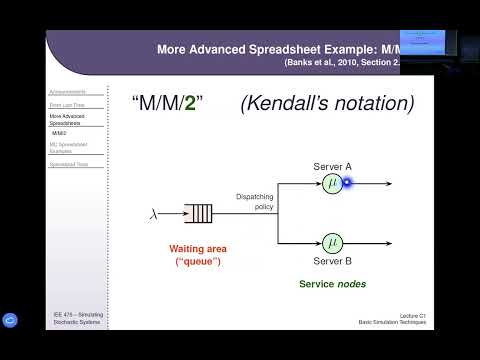
An M/M/2 queue has exponential interarrival times, exponential service times, and two servers with equal service rates.
Customers go to whichever server becomes available first; ties go to Abel, and customers wait if both servers are busy.
The spreadsheet adds server availability and service-completion columns to represent server state indirectly.

10:00 Spreadsheet Formulas for Server Assignment and Waiting

An IF formula assigns a customer to the server with the earlier availability time, with the tie rule assigning Abel first.
Service begins at the later of the arrival time and the earliest server-availability time, using a maximum operation to capture queueing delay.
For the selected server, service completion equals service start plus that customer’s sampled service time; the other server’s completion time carries forward.

16:00 Calculating Availability, Delay, and Time in System

A server becomes available for the next customer at the preceding completion time for that server.
Caller delay is service-start time minus arrival time; a customer arriving at 2 and starting at 4 waits 2 minutes.
Time in system is the selected server’s completion time minus the customer’s arrival time.

19:30 Queue Simulation Results and Steady-State Transients

A live queueing demo plots blue arrival ticks, red departure ticks, server service intervals, and the number of customers waiting.
Starting an M/M/1 queue empty creates a transient period with unusually short waits, so short-run averages can fall below steady-state predictions from IEE 470.
Longer runs or a warm-up period can bring simulation confidence intervals closer to steady-state results; simulations can also evaluate probabilities of exceeding a wait-time threshold.

29:00 Monte Carlo Methods: Random Sampling for Estimates

A Monte Carlo method uses repeated random sampling; a deterministic calculation that always returns the same output is not Monte Carlo.
One use estimates a fixed quantity, such as approximating π by randomized dart throws or estimating area with random rectangles.
Another use samples a stochastic model’s inputs, runs them through a simulation, and estimates the output distribution with a histogram.

31:00 Inventory Simulation and the Order-Up-To Policy

Inventory models often randomize demand at regular intervals, while the inventory remaining from one interval carries into the next.
An order-up-to policy checks inventory periodically and replenishes it toward a target level, subject to supplier lead time.
The decision balances shortage costs—such as lost sales or delayed orders—against holding costs such as warehouse space.

37:00 Using Cumulative Probabilities to Sample Demand and Lead Time

A demand table gives the probability of each daily order quantity; a separate lead-time distribution specifies how long replenishment takes.
Cumulative probabilities convert a uniform random number between 0 and 1 into an outcome; for example, a cumulative interval from 0.10 to 0.35 represents a 25% outcome.
The spreadsheet tracks beginning and ending inventory, shortages, pending order quantity, and days until delivery across 25-day runs.

44:00 Evaluating Inventory Outcomes Across Independent Runs

The example runs 100 independent 25-day blocks, then compares each run’s average daily ending inventory.
A distribution of inventory outcomes helps stakeholders judge whether they can afford to hold, for example, three or four refrigerators in stock.
The inventory widget varies order-up-to settings, holding charges, and back-order charges, and reports costs, shortage days, and success probabilities.

48:00 The Newsvendor Model and Profit Distributions

The newsvendor problem models perishable, fixed-price inventory such as newspapers: unsold stock loses its value after the selling period.
A more complex example samples both the type of day—good, fair, or poor—and the demand conditional on that day type.
Across 400 runs of 20 days, simulation produces a total-profit distribution that reveals downside risk and the chance of missing a minimum profit threshold.

52:00 Stretch Goals, Variance, and Bet Hedging

A stretch goal lies above the mean but within the range of achievable outcomes; a goal outside the distribution is not achievable under the modeled strategy.
When survival depends on clearing a high threshold, increasing variance can raise the probability of success even though it also increases the chance of very poor outcomes.
Ted Pavlic’s example contrasts a guaranteed $400 with a 50/50 chance of $0 or $800 when $500 is needed to pay rent; finance may seek asymmetric returns to expand upside without equally expanding downside.

58:00 Monte Carlo Simulation of Spatial Delivery Accuracy

A package-drop example samples landing locations from a bivariate normal distribution with standard deviations of 400 on the x-axis and 200 on the y-axis.
Success means landing inside an irregular target zone; a two-dimensional integral estimates the zone’s probability mass at about 69%.
Repeated simulations of 10 drops estimate the distribution of successful deliveries and the probability of meeting a threshold, such as at least nine packages in the zone.

1:04:00 Comparing Ball-Bearing Replacement Policies

A milling machine with three ball bearings fails when any bearing fails, creating a choice between replacing bearings individually, replacing all at failure, or adding scheduled replacement.
The model samples bearing lifetimes and repair delays, then accounts for bearing cost, mechanic cost, repair time, and downtime.
Repeated runs compare policy cost distributions; group replacement can reduce service calls but discards remaining bearing life, while scheduled replacement changes the downtime tradeoff.

1:11:00 Stochastic Activity Networks and the Central Limit Theorem

A stochastic activity network runs parallel paths—such as packing, paperwork, and inspection—and total completion time is determined by the slowest path.
Paths can have the same mean duration while having different distributions; sums of more activity times tend to become more bell-shaped.
The Central Limit Theorem helps explain why extreme total durations become less likely when several random activity times must be extreme together.

Summary, takeaways, and chapters were generated by AI from the video's transcript and may contain errors. The video belongs to its creator, Ted Pavlic.