IEE 475: Lecture B3 (2026-09-08): Discrete-Event Simulation Examples, Part II

Overview

Ted Pavlic connects discrete-event simulation mechanics to hands-on queueing and muffin-oven examples, distinguishing known activity durations from state-dependent delays and showing how events update system state. He also derives spreadsheet formulas for an M/M/1 queue and uses the muffin-policy experiment to explain Monte Carlo variability, common random numbers, blocking, paired t-tests, and why statistical significance must be weighed against practical significance.

Key takeaways

In a discrete-event model, an activity has a modeled duration and schedules its completion event, while a delay depends on system state and is terminated by an event.
For a single-server queue, service starts at max(customer arrival, previous service end); queue wait is service start minus arrival, and response time is service end minus arrival.
A spreadsheet can reproduce an M/M/1 hand simulation by expressing relationships among arrival, service-start, service-end, waiting, response, and idle-time columns.
Using common random numbers to compare two policies under the same ten demand schedules creates paired observations and reduces noise from differences between schedules.
A paired-difference t-test is a one-sample test of matched policy differences against zero; statistical significance alone does not establish that a change is practically worthwhile.
The best muffin-oven loading threshold depends on both demand and oven duration, so a policy that performs well for a three-minute bake may not be best for a seven- or fourteen-minute bake.

Chapters

0:00 Homework, Lab, and Midterm Timing

Homework B1 is due Saturday, while labs are due Sunday so solution sets can be available before midterm questions become restricted.
Homework B1 contains two questions plus a bonus; ICA1 is due before the next lecture.
Rockwell Arena competition entry forms for the fall session are due at the end of September.

2:00 Monte Carlo Lab 3: Estimating Pi and Output Distributions

Lab 3 introduces automated Monte Carlo runs, including estimating pi with random sampling and estimating an output distribution for a stochastic model.
The dart method estimates pi by the fraction of random points inside a circle inscribed in a square; that fraction approaches π/4.
Increasing the sample count to 5,000 tightens the estimates, while 95% confidence intervals across 100 trials illustrate run-to-run variability.
The Monte Carlo explorer also demonstrates Buffon's needle, robot path crossings as an area-estimation idea, and random integration under a curve.

6:26 Queueing Simulations: Activities Versus Delays

In the M/M/1 queue, interarrival and service-time distributions are known inputs, while customer waiting time emerges only after the system is simulated.
An activity is an unconditional wait with a modeled duration; a delay is conditional on system state and may vary with congestion.
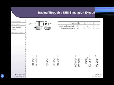
When customer C3 arrives while C2 is being served, C3's wait is not known until the server becomes available.
Simulation outputs such as response time help assess system-design choices, including adding servers in parallel or arranging them in sequence.

13:54 Events, Shared Resources, and State Changes

Limited shared resources create delays: examples include an airplane's single aisle, manufacturing equipment, and road intersections.
Starting an activity schedules a future primary event, such as the end of a customer's service.
Events can terminate delays: C2's departure makes the server available and can end C3's queue wait.
A state threshold can also trigger a conditional event, such as inventory reaching zero and scheduling six replacement refrigerators to arrive in six days.

18:00 Arrival and Departure Logic for Homework B1

On arrival, send a customer directly to the server if the checkout queue is empty; otherwise add the customer to the queue.
On departure, update the departure count and cumulative response time, calculated as departure time minus arrival time.
Homework B1 also tracks F, the count of customers whose response time is at least five time units.
If customers are waiting at a departure, start the next service and schedule its completion; otherwise the server remains idle.

23:54 Discrete-Event Terms and the Event Calendar

A system is the real-world process under study; a model is the representation used to answer what-if questions about it.
Discrete-event system state changes only at countable events, and the simulation clock advances to the next event notice in the future event list.
Entities can have attributes and be managed in lists, while the event calendar controls future events outside the model's ordinary entity lists.
Correct activity distributions matter because a proposed intervention may perform very differently under different input distributions.

28:00 Procedural, Object-Oriented, and Spreadsheet Simulation

Procedural languages such as C, Pascal, and BASIC represent simulation as imperative steps that manipulate program state.
Object-oriented languages such as C++, Java, and Swift encapsulate data and methods in interacting objects.
Spreadsheets are presented as declarative, cell-oriented data-flow systems: formulas specify relationships rather than an explicit sequence of steps.
The homework bonus asks students to use spreadsheet relationships to reproduce a hand-simulated M/M/1 queue without relying on spreadsheet state.

33:00 Spreadsheet Formulas for Arrivals and Service Starts

Compute each customer's arrival time as the previous arrival time plus that customer's interarrival time.
Compute service start as the maximum of the customer's arrival time and the previous customer's service-end time.
The MAX relationship captures both immediate service and waiting for the prior customer to finish.
Intermediate spreadsheet values may look wrong until dependent columns are completed, so formulas should be carried through before debugging results.

37:00 Deriving Queue Wait, Response Time, and Server Idle Time

Customer queue wait equals service-start time minus arrival time; a zero result means service began immediately.
Service-end time equals service-start time plus the customer's service duration.
Response time equals service-end time minus arrival time, so it includes both waiting and service.
For the single-server example, idle time is the nonnegative gap between the previous service end and the next service start, calculated with MAX(0, gap).

43:00 Validate Spreadsheet Results Against the Hand Simulation

The spreadsheet organizes customers down rows, while the hand simulation advances chronologically through events; both can produce matching departure times and response statistics.
For example, customer 3 arrives at time 6 and departs at time 13, yielding a seven-unit response time in both representations.
Spreadsheet formulas can reproduce a discrete-event trace, though managing large, general simulations this way would be tedious.
Changing interarrival or service-time inputs changes downstream results, demonstrating variability within a replication and between replications.

49:30 Muffin Simulation: Entity Granularity and Oven Policies

The Lab 2 muffin operation can model individual muffins or batches; batches simplify the model but may need to be split when they exceed oven capacity.
Entities can travel together, separate, and later reunite, as with family members at airport security or luggage separated from a passenger.
The greedy policy loads muffins immediately, while the nearly-full policy waits until enough muffins accumulate before using the oven.
The better policy depends on arrival rates and oven time: slow arrivals can make waiting costly, while rapid arrivals can make early, partial loads inefficient.

57:10 Statistical Versus Practical Significance in Policy Comparisons

A result from one muffin-demand schedule does not establish that greedy is generally better; comparisons across the ten ASU ID-based schedules show substantial variability.
Statistical significance asks whether observed differences could plausibly be random, while practical significance asks whether the improvement is valuable enough to justify its cost.
A difference such as 4.00 versus 4.15 minutes per muffin could be statistically detectable yet too small to matter operationally.
The appropriate test depends on experimental design: independent policy runs call for a two-sample t-test, while matched runs can support a paired analysis.

1:01:20 Common Random Numbers, Blocking, and Paired t-Tests

Lab 2 uses the same ten muffin-demand schedules for greedy and nearly-full policies, creating matched pairs rather than independent samples.
Using common random numbers blocks on demand schedule, helping separate the policy effect from schedule-to-schedule variation.
Across the paired schedules, nearly-full is generally slower than greedy; plotting within-schedule differences makes that pattern clearer than comparing unpaired averages.
A paired-difference t-test is a one-sample t-test on the ten differences against a zero mean; the reported result is statistically significant at p < 0.05.

1:08:20 Multiple Outputs, Linear Models, and Policy Interactions

Different outcomes can give different conclusions: time in system showed a significant policy difference, while oven utilization and maximum queue length did not.
Testing several outputs raises a multiple-comparisons issue; familywise error control and methods such as ANOVA or MANOVA are identified as later tools.
Varying oven-load thresholds beyond the greedy and nearly-full settings allows linear models to describe how a decision variable relates to performance.
The best threshold can depend on oven duration: the preferred policy can reverse as bake time rises from three to seven or fourteen minutes, illustrating an interaction.

Summary, takeaways, and chapters were generated by AI from the video's transcript and may contain errors. The video belongs to its creator, Ted Pavlic.