Fri Aug 28, 2026 Lecture (L03) Stewart Sections 1.4 (Calculating Limits) and 1.5 (Continuity).

Overview

Barsamian's Math Videos develops two calculus tools from Stewart Sections 1.4–1.5: the squeeze theorem for limits and continuity tests for functions and graphs. The lecture emphasizes how to apply theorems by checking every hypothesis, then uses the Intermediate Value Theorem to show that x^5 - x + 1 has a root in [-2, 2] and to frame a related existence question.

Key takeaways

To use the squeeze theorem, identify the approach point and three functions, verify the inequality near that point, and show both outer limits equal the same number before concluding the middle limit.
Continuity at a requires three checks: the two-sided limit exists, f(a) exists, and lim f(x) = f(a); the two-sided limit itself requires matching left- and right-hand limits.
A graph can have a cusp and still be continuous: at x = -3, the one-sided limits and function value are all 3, although the derivative fails to exist there.
Polynomials are continuous everywhere, while rational functions are continuous wherever defined; these facts justify direct substitution for their limits at points in their domains.
The Intermediate Value Theorem turns a sign change into a guaranteed root when the function is continuous: x⁵ - x + 1 has values -29 and 31 at -2 and 2, so it has a zero between them.

Chapters

0:00 Course Handout and the Return to Section 1.4 Limits

Lecture 3 follows the course calendar and revisits the limits handout from Wednesday before beginning Section 1.5 continuity.
The first topic is the squeeze theorem, a Section 1.4 tool not fully covered in the previous class.
The course webpage and calendar are available through Canvas, with lecture materials and handouts collected there.

2:00 Squeeze Theorem: Check Every Hypothesis Before the Conclusion

The theorem requires f(x) ≤ g(x) ≤ h(x) for x near a, possibly excluding a, and matching outer limits: lim f(x) = lim h(x) = L.
Under those conditions, lim g(x) = L as x approaches a.
Using a theorem means identifying its hypotheses and verifying each one; stating the conclusion alone does not establish the result.

6:00 Set Up the Squeeze Theorem for an Unknown Function

Example 1 gives -2x - 1 ≤ g(x) ≤ x² + 2x + 3 and asks for lim g(x) as x approaches -2.
The requested approach value identifies a = -2; the left and right bounds play f(x) and h(x), while g(x) is the unknown middle function.
The given inequality supplies the theorem's sandwich hypothesis, leaving the two outer limits to calculate.

10:00 Calculate the Outer Limits and Conclude the Limit Is 3

Direct substitution into the polynomial bound -2x - 1 at x = -2 gives 3.
Direct substitution into x² + 2x + 3 at x = -2 also gives 3.
Since both bounds approach 3 and the inequality holds, the squeeze theorem gives lim g(x) = 3 as x approaches -2.

16:00 Squeeze Trigonometric Expressions Near Zero

The lecture assigns the proof of lim x² sin(1/x) = 0 to Stewart Section 1.4, Example 9, which demonstrates the squeeze method.
For x² sin(1/x), the middle function is undefined at x = 0, but the squeeze inequality only needs to hold near zero, not at zero.
A parallel exercise is lim x⁴ cos(2/x) = 0; the class is directed to a similar worked example in the textbook.

25:00 Continuity at a Point as a Three-Part Test

The definition is f continuous at a when lim f(x) as x approaches a equals f(a).
The equality requires the limit to exist, f(a) to exist, and the two values to be equal.
To establish the two-sided limit, check that the left-hand and right-hand limits both exist and match.

30:00 Read Holes, Jumps, and Cusps Through Continuity

At x = 1, the graph approaches y = 3 from both sides, but the function value is missing; it passes the limit test and fails the function-value test.
At x = 4, the graph's limit is 1 while the plotted function value is 3, so the values do not match and continuity fails.
At x = -3, both one-sided limits and the function value are 3, so the cusp is continuous even though its derivative will not exist.

36:00 Continuity on Intervals and Familiar Function Families

A function is continuous on an interval when it is continuous at every point in that interval.
Polynomials are continuous everywhere, which explains why direct substitution works for polynomial limits.
Rational functions are continuous everywhere on their domains—at points where their denominators are nonzero.

40:30 Intermediate Value Theorem: From Endpoint Values to a Target

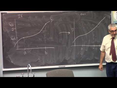
For a function continuous on [a, b], if f(a) and f(b) differ, every value strictly between them occurs as f(c) for some c in the interval.
A graph illustrates the result: a continuous curve connecting endpoint heights must reach each intermediate y-value.
As with the squeeze theorem, applying IVT requires verifying continuity, the interval, the endpoint values, and the target's position between them.

45:15 Apply IVT to Find a Root and Translate an Existence Question

For f(x) = x⁵ - x + 1 on [-2, 2], polynomial continuity satisfies the continuity hypothesis.
The endpoint calculations give f(-2) = -29 and f(2) = 31; since 0 lies between them, IVT guarantees a c in (-2, 2) with f(c) = 0.
The question of whether a number equals one more than its fifth power becomes x = x⁵ + 1, or x⁵ - x + 1 = 0; finding opposite signs at two inputs gives an IVT-based existence strategy.

Summary, takeaways, and chapters were generated by AI from the video's transcript and may contain errors. The video belongs to its creator, Barsamian's Math Videos.