fnb100f241007a

Overview

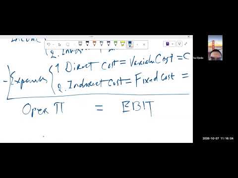
The class builds an income-statement sequence from sales revenue through operating profit (EBIT), earnings before taxes (EBT), and after-tax net profit (EAT). It connects accounting labels to production economics, explaining direct/variable costs and illustrating them with a Dell laptop example: $300 production cost and $500 selling price yield $3 million in costs and $5 million in revenue for 10,000 units.

Key takeaways

Sales revenue is calculated as price multiplied by quantity sold, making both selling price and sales volume explicit in the revenue calculation.
The income-statement progression taught is operating profit/EBIT, then EBT after interest expense, then net profit/EAT after taxes.
Interest expense reflects the cost of servicing borrowed capital; a manufacturer may need financing for plant and equipment before production can begin.
Total variable cost changes with quantity: at $300 per laptop, producing 10,000 units creates $3 million in production cost, while average variable cost remains $300 per unit.
For 10,000 laptops sold at $500 each and produced at $300 each, revenue is $5 million and COGS is $3 million.

Chapters

0:00 Class Opening and Review of the Income Statement

The class opens with attendance and a recap of the previous Monday’s lesson on income-statement structure.
The central purpose of the income statement is to show profit or loss from business activity.
The October 7 class is identified as section 5001.

3:00 Sales Revenue, Direct Costs, and Operating Expenses

Businesses earn revenue by making or selling goods and receiving payment from customers.
The lesson distinguishes direct costs, associated with production inputs, from indirect operating expenses, or OPEX.
Direct costs are compared with variable costs in microeconomics; operating expenses are compared with fixed costs.

9:30 Sales Revenue as Price Times Quantity Sold

Sales revenue is defined mathematically as selling price multiplied by quantity sold.
The formula avoids ambiguity in verbal descriptions such as “total amount of goods,” which do not specify the dollar value received.
The class uses price × quantity as the basis for later revenue and cost examples.

14:00 Operating Profit and the Meaning of EBIT

Subtracting business expenses from revenue produces operating profit, also called EBIT.
EBIT means earnings before interest and taxes, indicating that interest and tax payments have not yet been deducted.
Operating activity covers the process from selling goods or services through paying the costs required to produce them.

18:00 Why Borrowing Creates Interest Expense

Interest is treated as a business expense because it is the cost of servicing debt used to finance the business.
A computer manufacturer such as Dell needs substantial capital for plant and equipment before it can produce computers.
The lesson notes that startups may seek venture capital because banks rarely lend to startups; interest is deducted from EBIT to reach EBT.

26:00 EBT, Taxable Income, and After-Tax Net Profit

After interest is deducted from EBIT, the result is EBT: earnings before taxes, also called pre-tax profit or taxable income in the lesson.
Taxes are then deducted to arrive at net profit, also called net income or EAT (earnings after taxes).
The instructor recommends using “income” for gross income and “profit” for post-expense results to reduce confusion, while noting that accounting often uses income and profit interchangeably.

39:10 Production Inputs and the $300 Laptop Cost

The lesson identifies three production inputs: capital, labor, and raw materials.
Capital is illustrated by plant and equipment; computer raw materials include CPUs, GPUs, RAM, storage, keyboards, and screens.
A hypothetical Dell Model X laptop costs $300 per unit to produce, combining the costs of production inputs.

44:30 Variable Cost, Total Cost, and Average Variable Cost

At $300 per unit, producing 10 units costs $3,000, 100 units costs $30,000, and 10,000 units costs $3 million.
Total direct cost is called total variable cost because it changes with production quantity; zero units produce zero variable cost in the example.
Average variable cost is total variable cost divided by quantity, which returns the $300 unit production cost.

48:00 COGS and Revenue in the 10,000-Laptop Example

The lesson uses COGS (cost of goods sold) for total variable production costs associated with the units sold.
At a $500 selling price, 10,000 laptops generate $5 million in revenue; at $300 production cost each, COGS totals $3 million.
Revenue represents the selling-price side of the units sold, while COGS represents their cost side; the class also refers to this as cost of revenue.

52:00 Next Class: OPEX and the Monday Schedule on Tuesday

The next lesson will cover OPEX, or operating expenses.
Because of Columbus Day, the class will meet the following Tuesday at the usual time and follow Monday’s college schedule.
Tuesday-schedule classes will not meet that day; students are told to check the college calendar.

Summary, takeaways, and chapters were generated by AI from the video's transcript and may contain errors. The video belongs to its creator, Jeff Hunk.