ES.1802, October 6, 2026

Overview

The lesson connects Jacobian matrices to the multivariable chain rule, showing how derivatives compose across nested functions and how the same multiplication structure underlies backpropagation in neural networks. It then reviews tangent planes to implicitly defined surfaces, level surfaces and matrix transposes before expressing linear approximations in matrix notation and motivating quadratic Taylor approximations.

Key takeaways

A Jacobian for a mapping from n inputs to m outputs has dimensions m×n; each row contains the partial derivatives of one output with respect to all inputs.
For nested mappings, the multivariable chain rule is computed by multiplying Jacobians in dependency order, and a scalar-valued output produces a 1×n derivative row.
Neural-network backpropagation uses the chain rule across layers to calculate how changes in parameters affect the final output or error.
For an implicitly defined surface f(x,y,z)=c, the tangent plane at P is given by ∇f(P)·((x,y,z)−P)=0 because the gradient is normal to the level surface.
Writing a dot product as uᵀv makes its matrix dimensions explicit: a row vector times a column vector yields a 1×1 scalar.
The quadratic Taylor approximation adds second-derivative information to the linear approximation, capturing curvature and supporting local maximum/minimum analysis.

Chapters

0:00 Jacobian Dimensions for Vector-Valued Functions

For a function with components u and v depending on x and y, the Jacobian is a 2×2 matrix.
Each Jacobian row is the gradient of one output component: ∇u followed by ∇v.
With two outputs depending on x, y, and z, the Jacobian becomes 2×3, with one row per output and one column per input.

3:00 Composing Jacobians Through Nested Functions

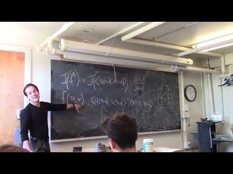
For dependencies (t,s) → (x,y) → (u,v) → f, the derivative from (t,s) to f is the product of the Jacobians at each layer.
The scalar-valued function f(u,v) has a 1×2 Jacobian, while the intermediate mappings can each have 2×2 Jacobians.
The resulting 1×2 row contains the two partial derivatives, df/dt and df/ds; multiplying the matrices expands into the sum over all dependency paths.

11:00 Backpropagation as the Chain Rule in Neural Networks

Training a neural network adjusts parameters to improve an output, such as reducing a model’s errors.
Backpropagation applies the chain rule through connected layers, multiplying local derivatives to determine how upstream parameters affect the final result.
The lesson’s nested-function example illustrates the same process: trace each dependency path, then combine its partial derivatives through matrix multiplication.

17:00 Implicit Surfaces and the Tangent-Plane Equation

For a surface defined implicitly by f(x,y,z)=constant, ∇f at a point is normal to the surface and therefore to its tangent plane.
The tangent plane can be written ∇f(P)·((x,y,z)−P)=0, avoiding the need to solve the surface equation explicitly for z.
For the sphere example, the point (1/√2, 1/√2, 1) gives gradient (√2, √2, 2) and tangent-plane equation √2x + √2y + 2z = 4.

27:00 Gradients, Normal Directions, and Level Surfaces

A gradient points toward the direction of greatest increase; for the sphere example, increasing the defining function moves outward to larger level surfaces.
A surface f(x,y,z)=c is a three-dimensional analogue of a two-variable level curve f(x,y)=c.
The tangent-plane normal may point either way, but ∇f specifically points toward increasing function values.

30:00 Matrix Transposes and Compatible Products

Transposing a 2×3 matrix produces a 3×2 matrix by turning each row into a column.
A matrix product is defined when the first matrix’s column count matches the second matrix’s row count; for example, a 3×2 matrix times a 2×3 matrix yields a 3×3 matrix.
Gradients are treated as column vectors in the upcoming linear-algebra notation, so their transposes are row vectors.

35:00 From Tangent Lines to Linear Approximations

Near a point p, a differentiable single-variable function is approximated by f(p) + f′(p)Δx.
In the multivariable case, the tangent-plane approximation to f(x,y) uses the gradient at p and the displacement from p.
This local approximation generalizes the familiar tangent-line estimate by incorporating changes in multiple input coordinates.

40:00 Writing the Gradient Approximation with Matrices

Vectors are represented as columns, so the dot product u·v is written uᵀv.
For two-dimensional inputs, ∇f(p)ᵀΔx is a 1×2 times 2×1 product, producing the scalar change used in the approximation.
The matrix form makes the linear approximation easier to extend from two variables to higher-dimensional inputs.

45:00 Quadratic Taylor Approximation and Curvature

A linear approximation captures nearby function values but does not describe curvature or concavity.
In one variable, the quadratic Taylor approximation adds ½f″(p)(Δx)² to f(p) + f′(p)Δx.
Second-order information helps distinguish local maxima and minima; its multivariable extension will involve a matrix.

Summary, takeaways, and chapters were generated by AI from the video's transcript and may contain errors. The video belongs to its creator, ChristianAltoSax.